CAM : a quality control pipeline for MNase-seq data
CAM is a quality control (QC) pipeline for MNase-seq data. By applying this pipeline, CAM uses either raw sequencing file or aligned file as an input (supporting both paired end and single end data; see our testing data and the Manual section for more information) and provides multiple informative QC measurements and nucleosome organization profiles on potentially functionally related regions for a given MNase-seq dataset. CAM also includes 268 historical MNase-seq datasets from human and mouse as a reference atlas for unbiased assessment.
Here, we provide an example to get you easily start in 3 steps on a Linux/MacOS system with only Python and R installed. You can use the default mode to run CAM with options specific to your data (see the Manual section for detailed usage).
Motivation:
Nucleosome organization affects the access of cis-elements to trans-acting factors. Micrococcal nuclease digestion followed by high-throughput sequencing (MNase-seq) is the most popular technology used to profile nucleosome organization on a genome-wide scale. Evaluating the data quality and focusing on potentially functionally related genomic regions remain challenging, especially for mammalian data. There is a strong need for a convenient and comprehensive approach to obtain dedicated quality control (QC) and to determine target regions for downstream analysis.
Results:
We developed CAM, which is a comprehensive QC for MNase-seq data. The CAM pipeline provides multiple informative QC measurements and nucleosome organization profiles on potentially functionally related regions for given MNase-seq data. CAM also includes 268 historical MNase-seq datasets from human and mouse as a reference atlas for unbiased assessment.
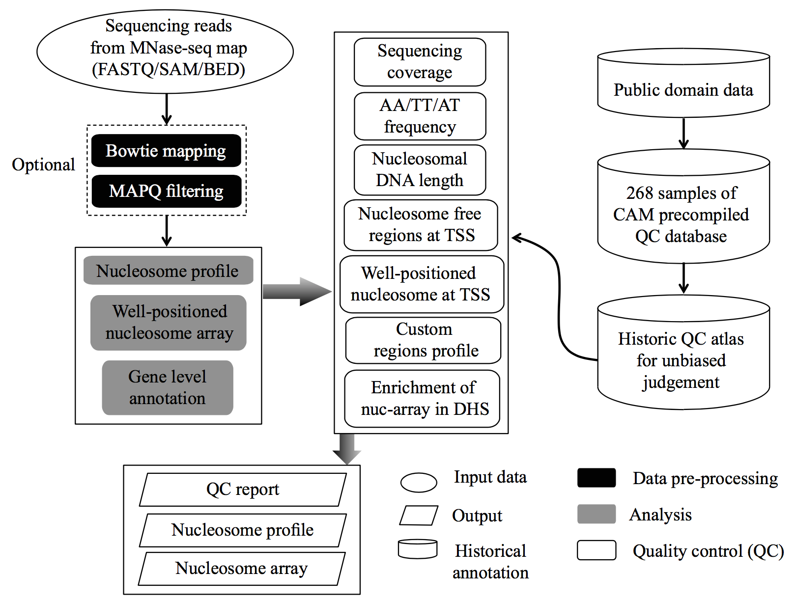
Workflow:
Citiation:
Manuscript under preparation
Contact:
If you have any questions, suggestions, bug reports, etc, feel free to contact :Shengen Hu(tarelahu@gmail.com)
Description
CAM is a QC pipeline for MNase-seq data. By applying this pipeline, CAM provides multiple informative QC measurements and nucleosome organization profiles on potentially functionally related regions for the given MNase-seq data. CAM also includes 268 historical MNase-seq datasets from human and mouse as a reference atlas for unbiased assessment. Here, we provide a detailed manual regarding the installation and usage of CAM. See the FAQ section if this section does not answer your questions.
Installation
Prerequire
1. python(version = 2.7)
2. R (version >= 2.14.1)
3. CAM will generate a summary QC report if you have pdflatex installed, otherwise you only get a package of QC plots and analysis results in the summary folder.
Install CAM
CAM uses Python's distutils tools for source installations. To install the CAM source distribution, unpack the distribution zip file and open up a command terminal. Go to the directory where you unpacked CAM and simply run the install script. We provide an example installation in the quick start section for users who are confused about the following description:
$ python setup.py install
By default, the script will install the python library and executable codes globally, which means you need to be the root or administrator of the machine to complete the installation. Please contact the administrator of the machine if you need help. If you need to provide a nonstandard install prefix or any other nonstandard options, you can provide many command line options to the install script. Use the --help option to see a brief list of available options.
$ python setup.py install --prefix /home/CAM
If you are not the root user, you will see “permission denied” when attempt to install CAM globally. Then, you can use --prefix parameter to install CAM to any directory in which you have write permission. You might need to add the install location to your PYTHONPATH and PATH environment variables. The process varies for each platform, but the general concept is the same across platforms.
Setup environment variables
PYTHONPATH
To set up your PYTHONPATH environment variable, you will need to add the value PREFIX/lib/pythonX.Y/site-packages to your existing PYTHONPATH. In this value, X.Y represents the major–minor version of Python you are using (for CAM it should be 2.7; you can find this with sys.version[:3] from a Python command line). PREFIX is the install prefix where CAM is installed. If you did not specify a prefix on the command line, CAM will be installed using the default Python system prefix. For example, if you specify the parameter “--prefix /home/CAM”, you must add /home/CAM/lib/python2.7/site-packages to your PYTHONPATH (below is an example, DO NOT add spaces around the equal sign).
$ export PYTHONPATH=/home/CAM/lib/python2.7/site-packages:$PYTHONPATH
PATH
Similar to PYTHONPATH, you will also need to add a new value to your PATH environment variable to use the CAM command line directly. Unlike the PYTHONPATH value, you will need to add PREFIX/bin to your PATH environment variable. The process for updating this information is the same as described above for the PYTHONPATH variable:
$ export PATH=/home/CAM/bin:$PATH
To check your default PATH and PYTHONPATH, you can type:
$ echo $PATH
$ echo $PYTHONPATH
Automatically export PATH and PYTHONPATH
Does exporting the environmental variables every time bother you?
In Linux, you can include the new values in your PYTHONPATH using bash by adding these lines:
$ export PATH=/home/CAM/bin:$PATH
$ export PYTHONPATH=/home/CAM/lib/python2.7/site-packages:$PYTHONPATH
to your ~/.bashrc (or ~/.bash_profile). Then, the environment is automatically exported, and you do not need to export the environment in the future.
Now you have CAM installed on your computer. Type
$ CAM.py --help
to check your installation.
Prepare genome sequence file
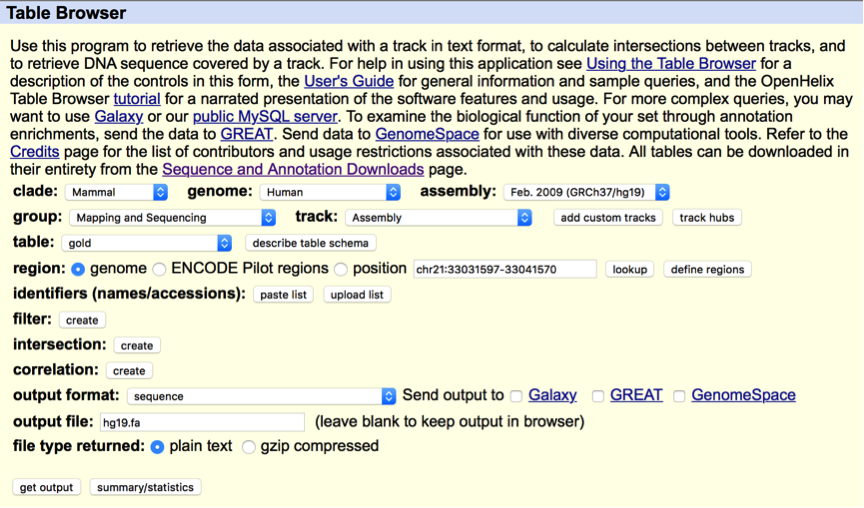
To conduct CAM, a genome sequence file in fasta (.fa) or 2bit (.2bit) is the ONLY required file. The genome sequence file is used for both the mapping step (optional) and the QC components, and can be downloaded from the UCSC genome browser http://genome.ucsc.edu/cgi-bin/hgTables. Below is an example of downloading the genome sequence file of the hg19 genome version from the UCSC genome browser.
We also provide download link in the Quick Start section.
Prepare bowtie mapping index files
This step is not required for CAM but can save processing time, especially when users have many MNase-seq samples to process. Users can build mapping index in advance, and input mapping index to CAM to avoid the step of generating mapping index, which is time consuming.
The parameter "--mapindex" should be the absolute path of index filename prefix (without trailing .X.ebwt). This parameter will be directly used as the mapping index parameter of bowtie.
eg: /home/user/bowtie_index/hg19 (then under your folder /home/user/bowtie_index/ there should be hg19.1.ebwt, hg19.rev.1.ebwt .... ).
CAM will generate bowtie index files in the annotation/ folder if the user run CAM with a genome sequence file in .fa format (eg. --fa hg19.fa) (turn off --clean parameter). User can backup the index generated and input to --mapindex in the next run.
Install pdflatex
MacOS users can get download "MacTex" from http://www.tug.org/mactex/. After downloading the package MacTex.pkg from http://tug.org/cgi-bin/mactex-download/MacTeX.pkg, double click to install MacTex and get the pdflatex.
For linux users, you can type
$ apt-get install texlive-allto install pdflatex on your server/computer.
Note that the installation of pdflatex on both the MacOS and Linux requires root privileges.
CAM Usage
An example mentioned in the Quick Start section
Now you can use the full functions of CAM, and the mapping index will be built automatically. See the following example with the CAM simple mode (see the example in the Quick Start section and the following section for the usage of the simple mode):
$ CAM.py simple -a GSM907784_1.fastq -b GSM907784_2.fastq -n GSM907784 -t PE -s hg19 --fa /home/data/hg19.fa -c /home/data/CTCF_motif_hg19.bed
# --fa /home/data/hg19.fa: absolute path of genome sequence file. Note that the genome version (-s hg19) should corresponded to the genome sequence (--fa /home/data/hg19.fa) file. The genome sequence file can be downloaded in the Download section.
# -c /home/data/CTCF_motif_hg19.bed: an example for custom regions in hg19 version. User can generate nucleosome profile on the custom region by specify this parameter. The example can be downloaded in the Download section.
Simple mode and Standard mode
CAM provides two modes. You can edit and design a parameter complex suitable for your data with the standard mode, but you need to generate a configure file and edit it before you start CAM. The simple mode is designed for convenience and a quick start. With this mode, you can run CAM with a simple command line, but only major parameters can be edited.
Simple mode
You may become familiar with the simple mode in the Quick Start section. In simple mode, you only need to specify the input data, output name, genome sequence, and species (genome version) with a command line. CAM will generate the QC and analysis results with all default parameters.
All parameters in simple mode are also in standard mode and are described below:
$ CAM.py simple [-h] -a INPUTA [-b INPUTB] -n NAME -s SPECIES -t {SE,PE} --fa GENOMESEQUENCE [-c CUSTOMREGION] [-p THREAD] [-f] [--clean]
Type
$ CAM.py simple -h
for a detailed description of all major parameters of the simple mode.
Standard mode
In standard mode you can edit all parameters and make CAM suitable for your data.
First you should generate a configure file by typing:
$ CAM.py gen your_config_name.conf
Now you have generated a configure file (named your_config_name.conf in the example). If you open the generated configure file, you will find all of the changeable parameters listed with the pattern "parameter = value" (for example, inputa = inputfile_1.fastq) and corresponding description at the bottom of each panel (starts with "#").
We use a Python package called “ConfigParser" to parse the configure file, which requires a specific pattern of the input configure file. Thus, user should be cautious when editing the configure file:
1. Do NOT edit the description lines (the lines start with "#"), these lines should start with "#"
2. Keep the pattern "parameter = value" for the parameter lines. Do NOT remove the value for any parameter line if you do not have a specific value for the line. The space next to the equal sign should be retained.
Now, you can edit your configure file and make it suitable for your MNase-seq data (If you don't know the suitable parameter at first time, try default parameters).
After you complete editing of the configure file, you can use standard mode to run CAM with your edited configure file as input.
CAM.py run -c your_edit_config.conf -f --clean
# -c your_edited_config.conf: name of your input configure file. The configure file should be generated from CAM gen mode or copied from the output of the other CAM run mode (described in the following sections). The major parameters (parameter with “[required]” in the description line) include the input file location, species, genome sequence, sequencing type and output name.
# -f: force_overwrite, CAM will overwrite the output result if the output folder already exists when -f is added. Otherwise, CAM will exit.
# --clean: CAM will remove the intermediate result if --clean is added.
DIY template configure file to save your specific parameters
If editing the configure file for the same parameters for each CAM run is too complicated, the template configure file can be edited in the CAM package prior to installation to save changes to some major parameters (e.g., edit species, genome_fasta and other parameters) in the template configure file. If you previously installed CAM, you can edit the template configure file and reinstall the program.
First, you should find the template configure file, which is located in the “lib/Config/” folder of the CAM package and named “CAM_template.conf” (do NOT change the file name of the template configure file).
After you find the template configure file, you can edit it to change some commonly used parameters. For example, if you change the parameter “species = hg19” in the template configure file, the configure file you generate next time will always have “species = hg19” and does not need to be reedited. Generally, we suggest editing the species and genome_fasta. You can also change other parameters for specific usages (after you know the usage of each parameter from the parameter section). The method used to edit the template configure file is similar to the method used to edit the generated configure file.
Both standard mode and simple mode can inherit the edits to the template configure file.
Full parameter description
Below is a description of all changeable parameters. The value after the equal sign is the default (suggested) value of the parameter. [required] means this parameter should be specified for different samples.
A more convenient method is to read the same version in configure file while you are editing configure file and specify the parameters.
General
# In General panel we describe major parameters of CAM
inputa =
inputb =
# [required]inputa: (ABSOLUTE path)main input file of CAM, accept FASTQ (raw MNase-seq data), SAM (bowtie alignment output) and BED (alignment output transformed from sam, 6 column, 5th column is bowtie map quality and 6th column is strand ) format, format is decided by the extension of input file(.fastq, .sam or .bed)
# inputb: (ABSOLUTE path)This parameter is for the 2nd part of paired-end FASTQ files. Required only if input file is FASTQ file and sequencing type is paired-end sequencing, only accept raw FASTQ file input. The extension should be .fastq. Note that if your data in paired end. User should also specify "seqtype"(below) as PE
seqtype = SE
# [required]seqtype: sequencing type of your sample, choose from SE(single end, default) and PE(paired end). Note that if you specify PE in seqtype and your data is FASTQ, you should give parameter to inputb. If your data is in SAM/BED (alignment) format, you don't need to specify inputb (it will be ignored if specified).
outputdirectory =
# [required]outputdirectory: (ABSOLUTE path) Directory for all result. Default is current dir "." (If was left blank) , but not recommended.
outname =
# [required]outname: Name of all your output results, your results will looks like outname.pdf, outname.txt
customregion =
# [optional]customregion: (ABSOLUTE path) user defined custom region to display nucleosome pattern.
# Custom region should be in absolute path, bed format and suffix should be .bed (e.g. /home/user/customregion/XXX.bed)
# Custom region require a 3 column bed or 6 column bed file, if it contains 6 or more columns, the 6th column should be strand (+/-), in that case CAM will display strand specific signal (e.g. flip signal for - strand).
# Limit of custom region is 50k, if the number of custom region is greater than 50k, CAM will take top 50k regions for nucleosome profile
# For example, user can input a list of motif sites (e.g. CTCF motifs) to check nucleosome pattern on certain motifs.
# Left this parameter empty if you don't need this function
Step1_preprocess
# In preprocess panel we describe parameters related to data process and transformation
mapping_p = 8
# mapping_p: Number of alignment threads to launch alignment software
genome_fasta = /home/user/genomefasta/hg19.fa
# genome_fasta: (ABSOLUTE path) whole genome sequence in FASTA format,
# The genome sequence should be in fasta format or 2bit format, genome_fasta file should be ends with .fa or .2bit and the genome version should be corresponding with -s species. This is the ONLY annotation file required for CAM
mapindex = /home/user/bowtie_index/hg19
# (ABSOLUTE path) mapindex: Mapping index of bowtie, absolute path,
# Users can build mapping index in advance, and input mapping index to CAM to avoid generating mapping index step, which is time consuming.
# bowtie mapindex should be absolute path of index filename prefix (without trailing .X.ebwt). this parameter will be directly used as the mapping index parameter of bowtie
# eg: --mapindex /home/user/bowtie_index/hg19 (then under your folder /home/user/bowtie_index/ there should be hg19.1.ebwt, hg19.rev.1.ebwt .... ),
species =
# species: you can input species name instead of download and specify gene_annotation & genome_length files. CAM can use build-in annotation files(gene_annotation, geonme_length) instead of user specified annotation files
# Note: by default CAM support hg19, hg38, mm9, mm10 as input for species
# Note: users can add custom species name, to do this, users can prepare gene annotation file and genome length file and add them into build-in folder, CAM can find corresponded annotation file in build-in packages.
# ***NOTE: CAM will ignore gene_annotation and genome_length if this parameter is set, no matter in template configure file or cmd line.
q30filter = 1
# q30filter: Use q30 criteria (Phred quality scores) to filter reads in SAM/BED files, set this parameter to 1(default) to turn on this option, set 0 to turn off. Default is 0 (turn off)
trim3end = 0
# trim3end: trim N bps from 3'end of each reads. Users can set e.g. 30bp to trim 30bp from 3'end of each reads.
# It takes effect when sequencing reads is too long (e.g. longer than library size).
# For longer reads, trim3end parameter can help trim adapter to improve mappability. Default: 0 (trim 0 bp == turn off).
# Note that for sam/bed input this parameter is ignored.
# CAM require fastq reads length consistent in same sample.
# Read_length - trim3nd should be greater than 18bp (at least 18bp should left for mapping, called lengh filter in following description).
# If trim3end == 0 (trun off), length filter is also close.
fragment_length_limit = 250
# [only works for PE data] fragment_length_limit: limit of fragment length. This parameter works for both bowtie mapping (-X, for FASTQ input) and mappable fragment length selection (for SAM/BED input)
rpm = 1
# rpm: normalize signal in profile bigwig to reads per million (RPM). set 1 to turn on (default) this function and set 0 to turn off
Step2_QC
# In QC panel we describe parameters related to QC and analysis measurements
sample_down_reads = 10000000
# sample_down_reads: randomly sample down 10M(default) reads to save time for some time consuming QC step, e.g. reads quality, nucleosome relationship, nucleosome length distribution
# You can change the sample down reads number by modify this parameter, also you can turn off sample down function by leave this parameter blank (time consuming~!).
upstreamtss = 1000
downstreamtss = 2000
# upstreamTSS/downstreamTSS: up/down stream distance to TSS for calculating reads TSS profile,
# By default we suggest 1000bp upstream (left in the aggregate plot) and 2000bp downstream (right in the aggregate plot), the limitation is 500bp up/down stream
reads_distance_range = 250
# reads_distance_range: for single end data, this parameter represent range of distance from each original reads 5'end to all downstream 3'end,
# For paired end data, this parameter represent range of fragment length, and should be same as "fragment_length_limit" in step1, default is 250bp
customregion_dis = 1000
# customregion_dis: distance to the center of each custom region to plot nucleosome profile, by default its 1000. User can modify this parameter but should be between 200 ~ 5000
# Note: this parameter will be ignored if customregion is not specified.
Step3_nucarray
# In nucarray panel we describe parameters related to detecting well-positioned nucleosome arrays
window_size = 70
# window_size: length(bp) of sliding window for Gaussian smoothing, 70 (default) means sliding window size is +-70 = 140bp
# Note: nucarray use wiggle track in 10bp step, so window size can only be 50, 60, and 70...
smooth_bandwidth = 30
# smooth_bandwidth: standard deviation (bps) for Gaussian smoothing, default is 30. See more detail in document.
array_fold = 2
# array_fold: fold change of array position score vs. background on each array, user can filter arrays by change this cutoff
array_length = 600
# array_length: minimum length of detected nucarray. CAM will discard all arrays with shorter length. By default its 600bp.
Output of CAM
We take an example for GSM907784 (mentioned in Getting started section) to display the detailed output of CAM.
After you finish CAM, find your results in the outname/summary/ folder.
OUTPUT LIST
Below is an example of output files (GSM907784 as example data).
| file name(size) | description | download link |
|---|---|---|
| GSM907784_summary.pdf (14M) | summary QC report of CAM | Google Drive Baidu Pan |
| GSM907784_profile.bw (4G) | genome-wide nucleosome profile | Google Drive Baidu Pan |
| GSM907784_Tss_profile.txt (21M) | nucleosome signal on promoter regions | Google Drive Baidu Pan |
| GSM907784_CustomRegion_profile.txt (4M) | nucleosome signal on custom regions | Google Drive Baidu Pan |
| GSM907784_Nucleosome_Array.bed (5M) | well-positioned nucleosome arrays | Google Drive Baidu Pan |
| GSM907784_geneLevel_nucarrayAnnotation.bed (3M) | gene level annotation of nucleosome arrays | Google Drive Baidu Pan |
| GSM907784_profile_on_Nucleosome_Array.bw(311M) | nucleosome signal on well-positioned nucleosome arrays | Google Drive Baidu Pan |
The details of QC measurements is shown blow:
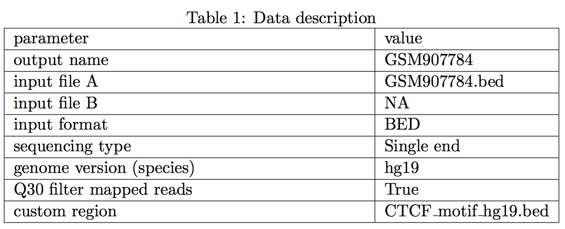
1 Data description
Table 1 mainly describe the input file and parameters for the CAM pipeline.
2 QC measurements
We provided multiple key measurements: 1) sequencing coverage, 2) AA/TT/AT di-nucleotide frequency, 3) nucleosomal DNA length, 4) existence of nucleosome free regions (NFR) at promoters, 5) well-positioned nucleosomes at downstream promoters, 6) well-positioned nucleosomes at custom defined potential cis-regulatory regions, 7) enrichment of well-positioned nucleosome arrays in DNase hypersensitive sites (DHS). The summary of the QC measurements and their judgments were listed in the table below.

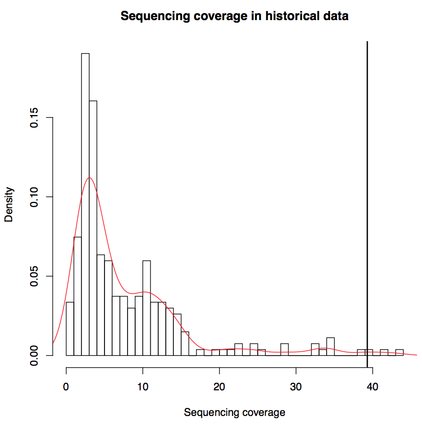
2.1 Sequencing coverage
Sequencing coverage provides a direct measurement of the resolution of two features of nucleosome organization, i.e. occupancy and positioning (Struhl and Segal, 2013). Sequencing coverage is defined as: (Number of reads * 194bp)/(Effective genome size). "Number of reads" is the number of mappable reads after MAPQ filtering. "194bp" is the total length of nucleosomal DNA and linker DNA estimated from historical data. "Effective genome size" is defined as 2.7e9 bp for human and 1.87e9 bps for mouse. Below we plotted the distribution of sequencing coverage of historical data; the sequencing coverage of the input data was marked by vertical line.
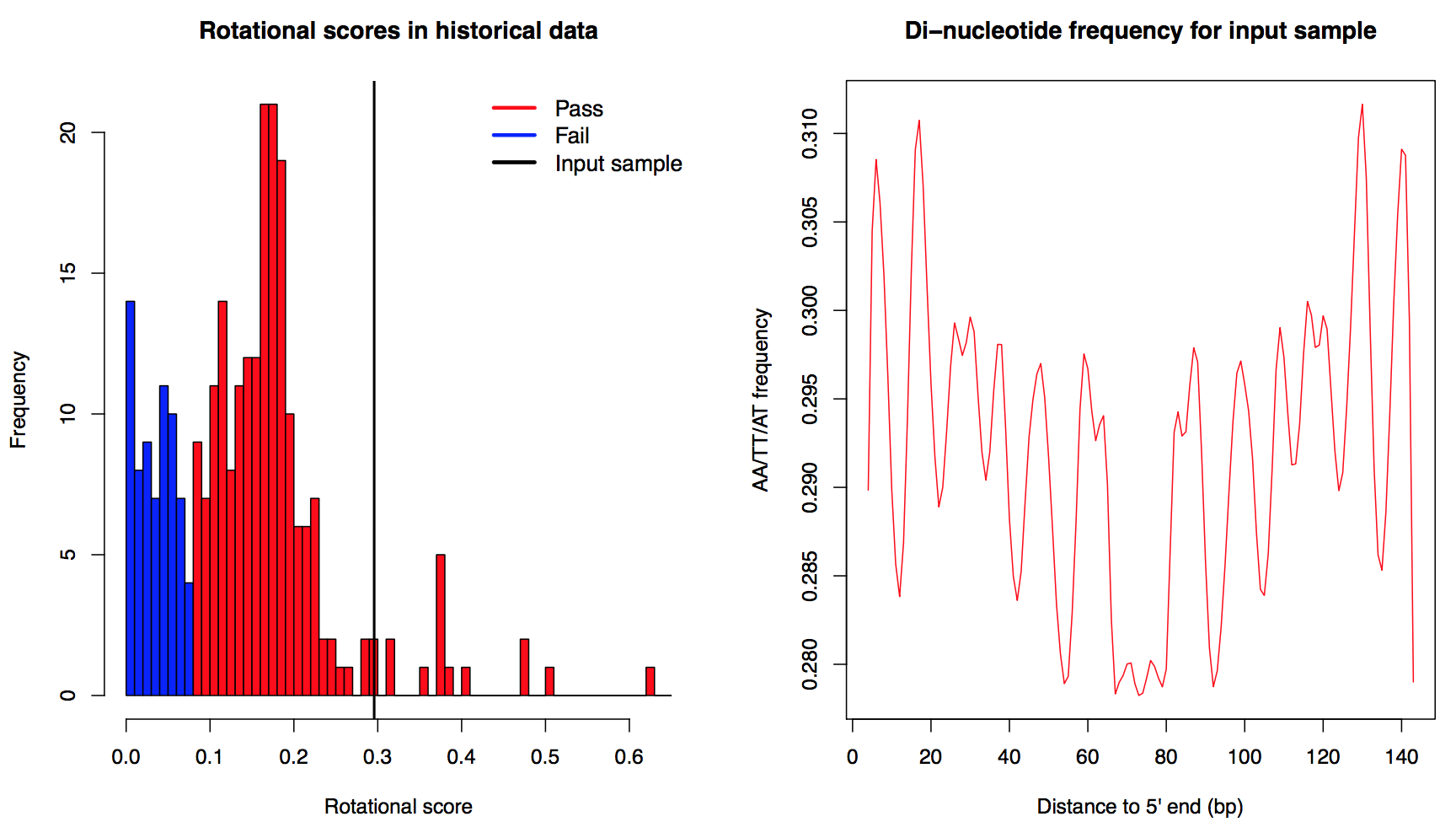
2.2 AA/TT/AT di-nucleotide frequency
The 10-base AA/TT/AT periodicity in nucleosomal DNA provides a measurement of nucleosome rotational positioning, which has been shown to be influenced by DNA sequence (Satchwell, et al., 1986). Mappable reads were sampled down to 10 million and were extended to 147 bp in their 3'end direction. Then the aggregate AA/TT/AT di-nucleotide frequency across 4th - 143th bp of the extended reads was calculated (right). We conducted a Fourier transform on the aggregate frequency and used the energy of 10-bp periodicity (defined as rotational score) to show the extent the MNase-seq reads reflect nucleosome organization. Samples with rotational score greater than 0.08 were defined as "Pass" in this measurement, otherwise they were defined as "Fail". The cutoff 0.08 was determined by the distribution of rotational scores from all historical data (left, vertical line marked the rotational score of the input sample.)
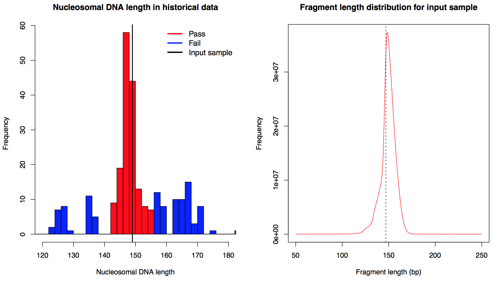
2.3 Nucleosomal DNA length distribution
Nucleosomal DNA length distribution (refer to fragment length or MNase library size) is closely related and thus can reflect the degree of MNase digestion. For paired end sample, fragment length distribution from all mappable fragments was used directly to infer the nucleosomal DNA length distribution. For single end sample, we calculated a start-to-end distance to estimate the nucleosome length: mappable reads were sampled down to 10 million and then we calculated the distribution of the distance from 5'end of each plus strand read to all 5'end of minus strand reads within 250 bp downstream. Duplicate reads were discarded in this calculation. After the distribution of nucleosomal DNA length was generated, the length with the highest frequency was defined as the estimated nucleosomal DNA length of the input sample (left, for both paired end and single end data). Samples with nucleosomal DNA length within 140bp - 155bp were defined as "Pass", otherwise they were defined as "Fail". The cutoff was determined by the distribution of nucleosomal DNA length from all historical data (left, vertical line marked the nucleosomal DNA length of the input sample.
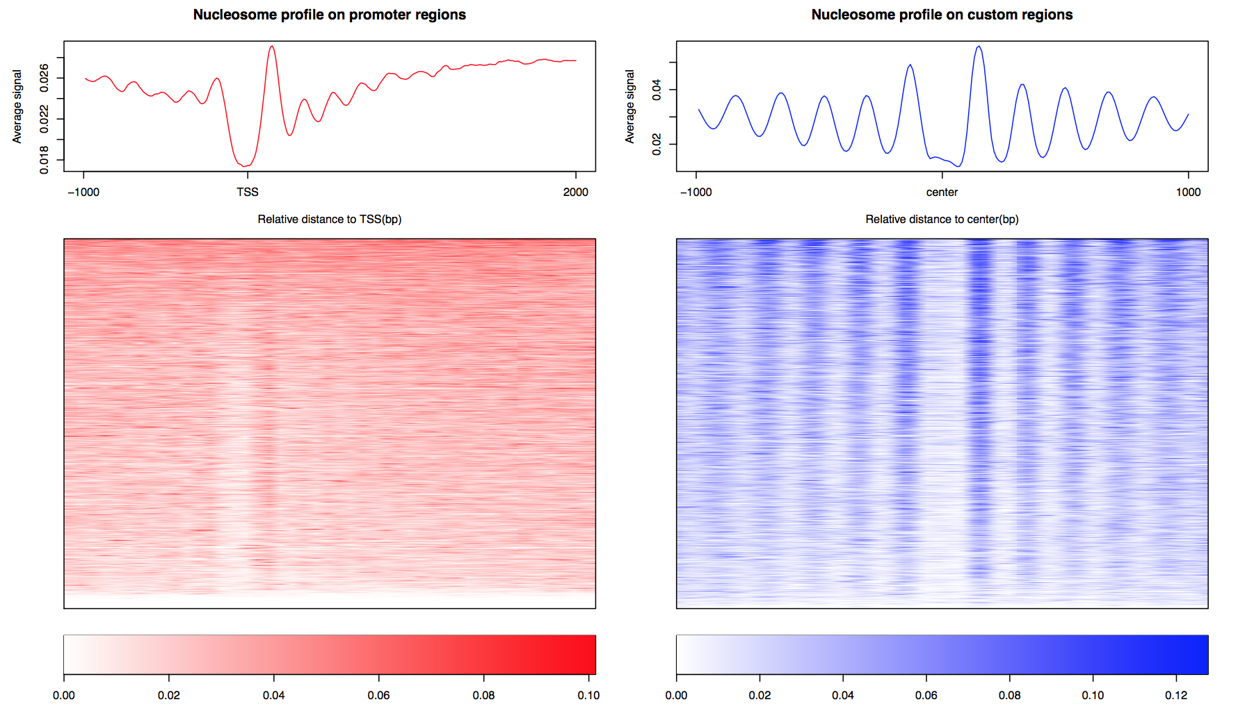
2.4 Nucleosome profile for potentially functional regions
CAM generated the aggregate curve and the heatmap of nucleosome organization on promoter regions and the custom regions: CTCF_motif_hg19.bed in 10 bp resolution. Signal from minus strand regions were reversed in both heatmap and aggregate curve. The signal for each region was also outputted as matrix: outputname_Tss_profile.txt & outputname_CustomRegion_profile.txt.
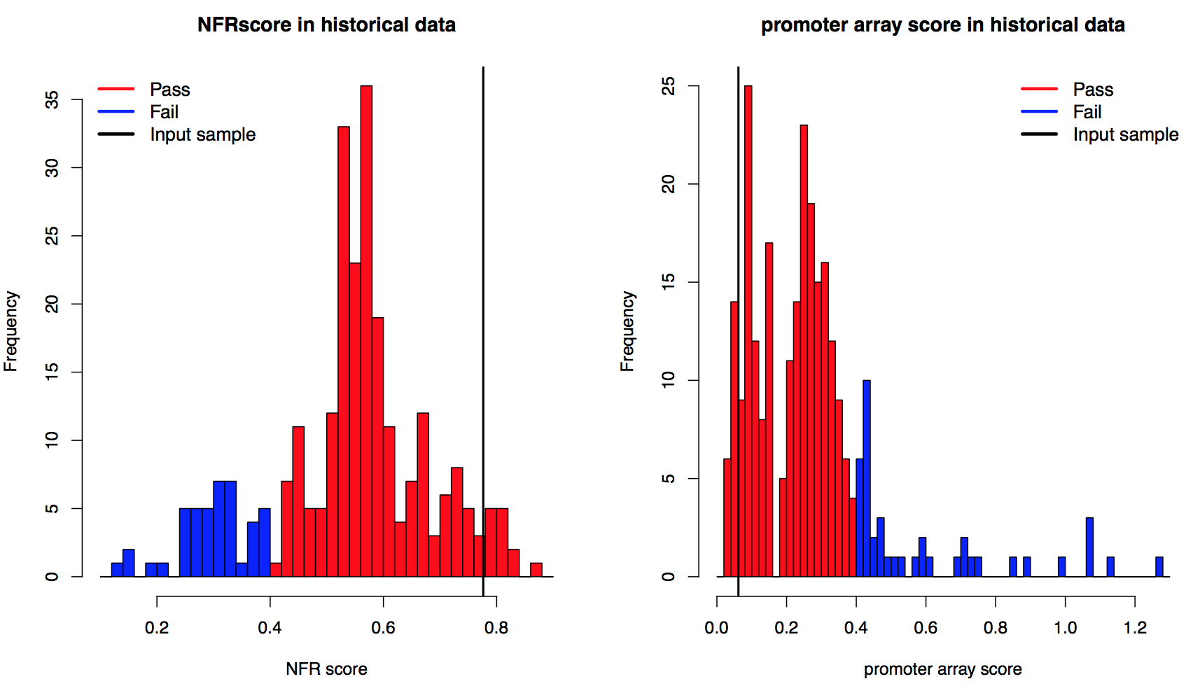
2.5 Nucleosome free regions (NFR) and nucleosome positioning on promoters
Based on nucleosome profile on promoters, CAM generated two scores to describe the nucleosome positioning on promoters. First, promoter NFR scores described the fold change of the MNase-seq signal of nucleosome free regions compared to the +1 nucleosome and -1 nucleosome. The higher the promoter NFR score is, the deeper the nucleosome free region is. Lower promoter NFR score associated with weak or none nucleosome free regions, which may indicate reads from open chromatins. Samples with promoter NFR scores higher than 0.4 were defined as "Pass", otherwise they were defined as "Fail".The cutoff was determined by the distribution of NFR scores from all historical data (left, vertical line marked the promoter NFR score of the input sample). Next, promoter nucleosome positioning score defined whether clear nucleosome positioning pattern was observed from downstream promoters. The promoter nucleosome positioning score was calculated by the coefficient of variance (CV) of the distance between the +1, +2, +3 and +4 nucleosomes. The lower the nucleosome positioning score is, the better nucleosome positioning was observed on downstream promoters. Samples with nucleosome positioning scores lower than 0.4 was defined as "Pass", otherwise they were defined as "Fail".The cutoff was determined by the distribution of nucleosome positioning scores from all historical data (right, vertical line marked the positioning score of the input sample).
2.6 Well-positioned nucleosome arrays
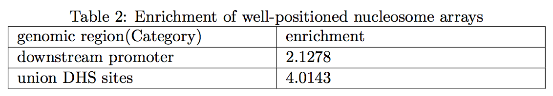
Regions with well-positioned nucleosome arrays were detected as previous described (Zhang, et al., 2014), and the enrichment in potential regulatory regions (downstream promoters and the union DNase I hypersensitive sites (DHS)) was listed. Enrichment was defined as observed/expected percentage of nucleosome array on promoters ( > 1 for enriched). Expected percentage was equal to the percentage of promoter length compared to the total length of effective genome. Similar approach was applied on the union DHS sites. For each region with well-positioned nucleosome array, its genomic coordinates together with the nucleosome profile value were reported in the output file: profile on Nucleosome Array. Samples with fold enrichment of DHS sites less than 2 were regarded as “Fail” in this measurement, indicating the well-positioned nucleosome arrays are more likely to be caused by random rather than the barrier nucleosome model. The gene level annotation of nucleosome arrays was also reported in output file: geneLevel nucarrayAnnotation (5th column represents overlapped nuc-array length)
Package download
CAM is implemented by Python and freely avialable : CAM.1.1.
macOSX version: CAM.1.1.macOSX.x86_64
Change log
v1.1.0 (2017.05.18) version 1.1, update for first plos one revision.
Genome sequence file download
We provide a convenient link for human (hg38 and hg19) and mouse (mm10 and mm9) genome sequences in twobit format from UCSC :hg38.2bit (size: 797M)
hg19.2bit (size: 778M)
mm10.2bit (size: 682M)
mm9.2bit (size: 680M)
If you can download genome sequence file from NONE of above links, you can also download genome sequence file from UCSC genome browser http://genome.ucsc.edu/cgi-bin/hgTables, see the Manual section.
Example of custom region file (CTCF motif sites in hg19, used in Quick start section):
CTCF_motif_hg19.bed (zip compressed)
Questions for downloading data
Q1: The links you provided for output result and the program are not downlaod link, I can't download directly.
A: Yes the links we provided are not direct link, you need to click to the webpage and click download yourself.
Q2: Why there's two copy of same links for output results?
A: Not totally same. For each of downloading file, we provide Google Drive link for users and Baidu Pan link as a backup, because Google Drive is not accessiable in some place.
Questions for CAM program
Q1: In your pipeline you use bowtie only as alignment tool, have you tried other alignment tool or at least bowtie2?
A: We tried many alignment tools and they show similar performance on most MNase-seq data, though some slight difference exist. The reason we use bowtie1 is because we prefer the unique aligned function of bowtie1 (-m 1, which is no longer exist in bowtie2). We mentioned in the manual section that users can align their MNase-seq data with their prefered software and input the result (SAM format recommended) to CAM and take the following function.
Q2: Followed Q1, bowtie1 don't output mapping quality (MAPQ) when -m 1 is turned on, but CAM still have Q30 filter function. Is this a bug?
A: We understand that bowtie1 only report 0/255 for uniquely map (-m 1) mode. However, q30 is also effective in separating reads with quality=0 or 255 which helps remove non-uniquely mapped reads. What's more, q30 also works for aligned reads (SAM/BED) input which is aligned by other aligner user prefered.
Q3: What should I do if I do want to generate your example output myself?
A: If you want to generate our example output yourself, you can download the corresponded MNase-seq data from GEO (accession ID: GSM907784), annotation file (hg19) and custom region file in the Download section. Then you run CAM with all default parameters to get the example results (you can use both simple mode and standard mode with hg19 as genome version). NOTE that GSM907784 has 4 parts of .sra file, user should download all 4 parts, transform to paired end fastq, and combine them for CAM input. User can also input single part only, in which case the output result will be slightly different.
Q4: The published MNase-seq data I download is not in FASTQ format, but .sra format ?
A: If you download the MNase-seq from public domain (say, GEO), you will get a .sra file. Then you can transform the .sra file to FASTQ format with a free software called fastq-dump (from package SRA toolkit http://www.ncbi.nlm.nih.gov/Traces/sra/sra.cgi?view=software ). After you successfully installed SRA toolkit, Type command line:
$ fastq-dump.2.2.2 --split-files SRRXXXXX.sraThen the .sra file will be split to 1 FASTQ files (for paired end there are 2 FASTQ files), named as SRRXXXXX_1.fastq and SRRXXXXX_2.fastq (paired end) or SRRXXXXX.fastq (single end).
Q5: I don't have pdflatex, and I don't have root permission to install it. How can I get the CAM QC report?
A: CAM will still process and generate all results without pdflatex, you can check summary/ folder for everything you want. Also, if you do need the summary report, you can copy the summary/plots/ folder to another machine with pdflatex installed and type:
$ pdflatex outname_summary.tex
In the summary/plots/ folder to generate the summary report.
Q6: The pipeline take too much time, its too slow !
A: Actually CAM take very little time to generate QC report and analysis results. The most time consuming step (which take more than 80% of time) is the mapping step, because MNase-seq data usually have deep sequencing coverage. Users can modify -p parameter to speed up the mapping step. User can also specify mapping index to skip bowtie-build step (which take time to generate bowtie mapping index).