quality control and analysis for Drop-seq
Dr.seq is a QC and analysis pipeline for Drop-seq data. By applying this pipeline, Dr.seq takes two sequencing files as input (data_1.fastq for barcode information, data_2.fastq for reads information, see our testing data and Manual section for more information) and provides four groups of QC measurements for given Drop-seq data, including reads level, bulk-cell level, individual-cell level and cell-clustering level QC.
Here we provide an example to get you easily started on a linux/MacOS system with only python and R installed. You can use standard mode to run Dr.seq with options specific to your data (see Manual section for detailed usage).
Motivation:
Drop-seq has recently emerged as a powerful technology to analyze gene expression from thousands of individual cells simultaneously. Currently, Drop-seq technology requires refinement, and quality control (QC) steps are critical for such data analysis. There is a strong need for a convenient and comprehensive approach to obtain dedicated QC and to determine the relationships between cells for ultra-high-dimensional data sets.
Results:
Dr.seq is a QC and analysis pipeline for Drop-seq data. By applying this pipeline, Dr.seq provides four groups of QC measurements for given Drop-seq data, including reads level, bulk-cell level, individual-cell level and cell-clustering level QC. We assessed Dr.seq on simulated and published Drop-seq data. Both assessments exhibit reliable results. Overall, Dr.seq is a comprehensive QC and analysis pipeline designed for Drop-seq data that is easily extended to other droplet-based data types.
Workflow:

The workflow of the Dr.seq pipeline includes QC and analysis components. The QC component contains reads level, bulk-cell level, individual-cell level and cell-clustering level QC.
Citiation:
Huo Xiao, Sheng’en Hu, Chengchen Zhao, and Yong Zhang. Dr. seq: a quality control and analysis pipeline for droplet sequencing. Bioinformatics (2016): btw174.
Contact:
If you have any questions, suggestions, bug reports, etc, feel free to contact :Shengen Hu(tarelahu@gmail.com)
Installation
Prerequisite
1. python(version = 2.7)
2. R (version >= 2.14.1)
3. Dr.seq will generate a summary QC report if you have pdflatex installed, otherwise you only get a package of QC plots and analysis results in the summary.
Install Dr.seq
Dr.seq uses Python's distutils tools for source installations. To install a source distribution of Dr.seq, unpack the distribution zip file and open up a command terminal. Go to the directory where you unpacked Dr.seq, and simply run the install script (We provide an example for installation in quick start section for users who feel confusing about the following description.):
$ python setup.py install
By default, the script will install python library and executable codes globally, which means you need to be root or administrator of the machine so as to complete the installation. Please contact the administrator of that machine if you want their help. If you need to provide a nonstandard install prefix, or any other nonstandard options, you can provide many command line options to the install script. Use the --help option to see a brief list of available options.
$ python setup.py install --prefix /home/drseq
If you are not root user, you will be mentioned “permission denied” when you tried to install Dr.seq globally. Then you can use --prefix parameter to install Dr.seq to any directory you have write permission, you might need to add the install location to your PYTHONPATH and PATH environment variables. The process for doing this varies on each platform, but the general concept is the same across platforms.
Setup environment variable
PYTHONPATH
To set up your PYTHONPATH environment variable, you'll need to add the value PREFIX/lib/pythonX.Y/site-packages to your existing PYTHONPATH. In this value, X.Y stands for the major–minor version of Python you are using (in Dr.seq it should be 2.7; you can find this with sys.version[:3] from a Python command line). PREFIX is the install prefix where you installed Dr.seq. If you did not specify a prefix on the command line, Dr.seq will be installed using Python's sys.prefix value.
For example, if you specify the parameter “--prefix /home/drseq”, you have to add /home/drseq/lib/python2.7/site-packages to your PYTHONPATH (below is an example, DON’T add space near the equals sign).
$ export PYTHONPATH=/home/drseq/lib/python2.7/site-packages:$PYTHONPATH
PATH
Just like your PYTHONPATH, you'll also need to add a new value to your PATH environment variable so that you can use the Dr.seq command line directly. Unlike the PYTHONPATH value, however, this time you'll need to add PREFIX/bin to your PATH environment variable. The process for updating this is the same as described above for the PYTHONPATH variable:
$ export PATH=/home/drseq/bin:$PATH
To check your default PATH and PYTHONPATH, you can type:
$ echo $PATH
$ echo $PYTHONPATH
Automatically export PATH and PYTHONPATH
Feel bothering export environment variable every time ?
On Linux, using bash, you can include the new value in my PYTHONPATH by adding these lines
$ export PATH=/home/drseq/bin:$PATHto your ~/.bashrc (or ~/.bash_profile). Then you export environment automatically and don’t need to export environment next time.
$ export PYTHONPATH=/home/drseq/lib/python2.7/site-packages:$PYTHONPATH
Now you have Dr.seq installed on your computer, type “Dr.seq --help” to check your installation.
Prepare gene annotation file
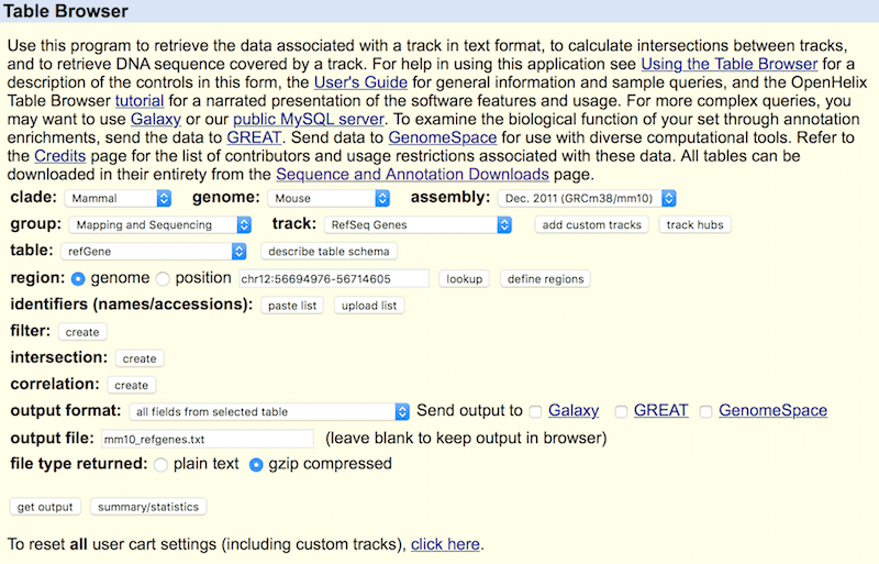
To conduct Dr.seq, a gene annotation file is required for the information of the location, name and composition of each gene. Dr.seq requires gene annotation file in full information format downloaded from UCSC genome browser http://genome.ucsc.edu/cgi-bin/hgTables. Below is an example for downloading gene annotation file from UCSC genome browser in mm10 genome version.
We suggest to use refseq genes as gene annotation, but you can also use annotation from other database.
Prepare alignment software and build index
After you installed Dr.seq on your computer, you can handle Drop-seq data with barcode file in FASTQ format and reads file in SAM format (reads file is pre-aligned to corresponded genome by any aligner). If you want to use the full function of Dr.seq (including alignment step, that is, users can just input raw barcode file and raw reads file in FASTQ format and get QC and analysis results back), you should install alignment software in your default PATH and build index yourself.
In Dr.seq we accept STAR(default) and bowtie2 as aligner.
We provide download link for executable alignment software and mapping index to save time and effort, see the following description and download section.
1. Install STAR and build STAR index
By default we use STAR (version >= 2.5.0) as alignment software because of its speed and performande, but STAR also consume great memory size. To use STAR for alignment in Dr.seq, first you should make sure the memory of your server is greater than 40G. Dr.seq will check the total memory of your server before alignment step if you chose STAR as alignment software (see the parameter description section for corresponded parameter: checkmem). We don’t suggest users to run STAR on a Mac.
To install STAR on you server, first you should download STAR package and install STAR according to their manual (github for STAR: https://github.com/alexdobin/STAR)
If you don’t want to or have trouble install STAR, we provide download link for executable STAR compiled in linux_x86_64 and macos_x86_64 system. See the download section of our webpage.
After you successfully install STAR or download executable STAR, the next step is to build STAR index. If you don’t want to or have trouble build STAR index, we provide download link for STAR index in different species and genome versions, including hg38, hg19, mm10, mm9. See the download section of our webpage.
To build STAR index first you have to download genome assembly file (regularly its .fa file, you can easily download it from UCSC genome browser http://genome.ucsc.edu/cgi-bin/hgTables , below is an example for downloading genome sequence in FASTA/fa format in mm10 genome version)

After you download genome .fa file, what you need is to run a STAR build command to transform your .fa file to an index package (note that to you have to create the directory yourself before you build STAR index).
$ mkdir /home/user/STAR_index# --runMode genomeGenerate: choose STAR build-index mode
$ STAR --runMode genomeGenerate --genomeDir /home/user/STAR_index --genomeFastaFiles /home/data/mm10.fa --runThreadN 8
# --genomeDir /home/user/STAR_index: name of directory you build STAR index in
# --genomeFastaFiles /home/data/mm10.fa: the genome .fa file you just download from UCSC
# --runThreadN 8: how many thread you want to use to generate STAR index, it's a speed up parameter
After you finish index building, you can use STAR as aligner in Dr.seq simple mode (see the example in Quick Start section for the usage of simple mode)
$ Drseq.py simple -b SRR1853178_1.fastq -r SRR1853178_2.fastq -n GSM1626793_mouse_retina1 -g /home/user/annotation/mm10_refgenes.txt --maptool STAR --mapindex /home/user/STAR_index
Note that “STAR” is case sensitive in --maptool parameter. In another word, Dr.seq will exit and let you input correct alignment software if you want to conduct alignment step and input “--maptool star” as a parameter. The directory in which you generate STAR index is just the parameter of --mapindex
Here the parameter -g, --mapindex should be inputed with absolute path.
2. Install bowtie2 and build bowtie2 index
If your server/computer don’t have more than 40G memory (for example, you want to run Dr.seq on a Mac), you can use bowtie2 (version 2.2.6) as an aligner instead, because bowtie2 consume less memory (< 3G memory for human genome) though slower. And that’s also the reason we use bowtie2 for Quick Start (another reason is that the index of bowtie2 is smaller and take less time to download).
You may already get familiar with in the Quick Start section. Similar like STAR, you can download and compile bowtie2 according to the manual from bowtie2 website (http://bowtie-bio.sourceforge.net/bowtie2/manual.shtml).
If you don’t want to or have trouble install bowtie2 and build bowtie2 index, we provide download link for executable bowtie2 compiled in linux_x86_64 and macos_x86_64 system and bowtie2 index in different species and genome version. See the download section of our webpage.
Bowtie2 has its own index. After you finish installing bowtie2, you can use bowtie2-build command to build bowtie2 index.
$ mkdir /home/user/bowtie2_index
$ cd /home/user/bowtie2_index
$ bowtie2-build mm10.fa mm10
After you finish index building, you can use bowtie2 as aligner in Dr.seq simple mode (see the example in Quick Start section for the usage of simple mode)
$ Drseq.py simple -b SRR1853178_1.fastq -r SRR1853178_2.fastq -n GSM1626793_mouse_retina1 -g /home/user/annotation/mm10_refgenes.txt --maptool STAR --mapindex /home/user/bowtie2_index/mm10# --mapindex /home/user/bowtie2_index/mm10: absolute path of bowtie2 index. Note that the genome version of the index should corresponded to the annotation file. If you have an index file looks like: /home/user/bowtie2_index/mm10.1.bt2, the red part is the one you should input here.
Install pdflatex
For mac user, you can get download “MacTex” from http://www.tug.org/mactex/. After downloading the package MacTex.pkg from http://tug.org/cgi-bin/mactex-download/MacTeX.pkg, you just double click to install MacTex and get the pdflatex.
For linux user, you can type
$ apt-get install texlive-allto install pdflatex on your server/computer.
Note that the installation of pdflatex on both mac and linux requires root privilege.
Usage of Dr.seq
Standard mode and simple mode
Dr.seq provides two modes, you can edit and design a parameter complex suitable for your data with standard mode but you need to generate a configure file and edit it before you start Dr.seq. Simple mode is designed for convenience and quick start. With this mode, you can run Dr.seq with a simple command line, but you can only edit major parameters with this mode.
Simple mode
You may get familiar with simple mode in the quick start section. In simple mode you only need to specify input data, output name, mapping tool, annotation and mapping index with a command line and Dr.seq will generate QC and analysis reports with all default parameters.
All parameters in simple mode are also in standard mode and will be described below:
$ Drseq.py simple [-h] -b BARCODE -r READS -n NAME[--cellbarcodelength CBL] [--umilength UMIL] [-g GA][--maptool {STAR,bowtie2}] [--checkmem {0,1}][--mapindex MAPINDEX] [--thread P] [-f] [--clean][--select_cell_measure {1,2}][--remove_low_dup_cell {0,1}]
Type$ Drseq.py simple -hfor detailed description of all major parameters of simple mode.
Standard mode
In standard mode you can edit all parameters you want and make Dr.seq suitable for your data.
First you should generate a configure file according to the template configure file (we will describe how to find and edit template configure file below) by typing:
$ Drseq.py gen your_config_name.conf
Now you have generated a configure file (named your_config_name.conf in the example) according to the template configure file. If you open the configure file you just generated you will find all changeable parameters listed with the pattern “parameter = value” (for example, barcode_file = SRR1853178_1.fastq) and corresponded description in the bottom of each panel (starts with “#”).
We use a python package called “ConfigParser” to parse configure file, which required specific pattern of input configure file. So user have certain caution when editing configure file:
1. Don't edit the description lines (the lines start with “#”), keep these lines start with “#”
2. Keep the pattern “parameter = value” for parameter lines. Don’t remove value for any parameter line if you don’t have specific value for it. And keep the space next to the equal sign.
Now you can edit your configure file and make it suitable for your Drop-seq data (If you don’t know the suitable parameter at first time, you can run Dr.seq simple mode with only major parameters changed and edit other parameters according to the performande of Dr.seq output, then you can re-run Dr.seq with updated parameters, the re-run of Dr.seq only take 20% of total time, see FAQ section).
After you finish configure file editing, you can use standard mode to run Dr.seq with your edited configure file input.
Drseq.py run -c your_edit_config.conf -f --clean# -c your_edited_config.conf: name of your input configure file, the configure file should be generated from Drseq.py gen mode or copy from other Drseq run. The major parameters (parameter with “[required]” in the description line) including input file location, gene annotation file location, alignment software and mapping index corresponded to the software should be specified by user.
# -f: force_overwrite, Dr.seq will overwrite output result if the output folder already exist when -f is added, otherwise Dr.seq will exit.
# --clean: Dr.seq will remove intermediate result if --clean is added.
DIY template configure file to save your specific parameters
If it’s too complicated for you to edit configure file for same parameters for each Dr.seq run. You can edit the template configure file in the Dr.seq package before you install Dr.seq, to save your changes for some major parameters (for example, edit gene annotation file, alignment software, mapping index and other parameters) in the template configure file. If you have already installed Dr.seq, you can edit the template configure file and install again.
First you should find the template configure file. It locates in the “lib/Config/” folder of Dr.seq package and named as “Drseq_template.conf” (do NOT change the file name of the template configure file).
After you find the template configure file, you can edit it to change some commonly used parameters. For example if you change parameter “gene_annotation = /data/mm10_refgenes.txt” and then re-install Dr.seq, the configure file you generate next time will always has “gene_annotation = /data/mm10_refgenes.txt” and you don’t need to edit it again. Generally we suggest editing gene_annotation, mapping_software_main and mapindex. You can also change cell_barcode_length if your barcode looks different from the published Drop-seq data (12bp for cell barcode, 8bp for UMI). The way you edit template configure file is similar like editing generated configure file.
Both standard mode and simple mode can inherit your editing on the template configure file.
Full parameter description
Below is the description of all changeable parameters. The value after equal sign is the default (suggested) value of the parameter. [required] means this parameter should be specified for different samples.
A more convenient way is to read the same version in configure file while you are editing configure file and specify parameters.
General
# In General panel we describe major parameters of Dr.seq
barcode_file = /home/user/SRR1853178_1.fastq
# [required]barcode_file : Fastq file only, by default, every barcode in fastq file consist of 20 bp including 12bp cell barcode(1-12bp) and 8bp UMI(13-20bp). Cell barcode should locate before UMI, the length of cell barcode and UMI can be defined below.
# eg: /home/user/SRR1853178_1.fastq
cell_barcode_length = 12
umi_length = 8
# cell_barcode_length/umi_length: Length of cell barcode and UMI, (see the annotation of barcoe_fastq). By default they are 12,8, respectively
reads_file = /home/user/SRR1853178_2.fastq
# [required]reads_file: Accept raw sequencing file (fastq) or aligned file(sam), file type is specified by extension. (regard as raw file and add mapping step if .fastq, regard as aligned file and skip alignment step if .sam), sam file should be with header.
# eg: /home/user/SRR1853178_2.fastq
outputdirectory = /home/user/GSM1626793_mouse_retina1/
# [required]outputdirectory: (absolute path) Directory for all result. Default is current dir "." if user left it blank , but not recommended.
# eg: /home/user/GSM1626793_mouse_retina1/
outname = GSM1626793_mouse_retina1
# [required]outname: Name of all your output results, your results will looks like outname.pdf, outname.txt
# eg: GSM1626793_mouse_retina1
gene_annotation = /home/user/annotation/mm10_refgenes.txt
# [required]gene_annotation: (absolute path) Gene model in full text format, download from UCSC genome browser,
# eg: /yourfolder/mm10_refgenes.txt (absolute path, refseq version recommended )
png_for_dot = 0
# png_for_dot: Only works for dotplots in individual cell QC. Set 1 to plot dotplots in individual cell QC in png format, otherwise they will be plotted in pdf format. The format of other plots is fixed to pdf.
# Make sure your Rscript is able to generate PNG plots if you turn on this function.
Step1_Mapping
# In Mapping panel we describe parameters related to the alignment of reads file
mapping_software_main = STAR
# [required if reads file is FASTQ format]mapping_software_main: name of your mapping software, choose from STAR and bowtie2 (case sensitive), STAR (bowtie2) should be installed in your default PATH
checkmem = 1
# checkmem: (only take effect when mapping_software_main = STAR) Dr.seq will check your total memory to make sure its greater 40G if you choose STAR as mapping tool. We don't suggest running STAR on Mac. You can turn off (set 0) this function if you prefer STAR regardless of your memory (which may cause crash down of your computer)
mapping_p = 8
# mapping_p: Number of alignment threads to launch
mapindex = /home/user/STAR_index
# [required if reads file is FASTQ format]mapindex: Mapping index of your alignment tool, absolute path,
# Mapping index should be built before you run this pipeline, note that STAR and bowtie2 use different index type (see STAR/bowtie2 document for more details.).
# For STAR, mapindex should be the absolute path of the folder you built STAR index, this parameter will be directly used as the mapping index parameter of STAR
# eg: /mnt/Storage3/mapping_idnex/mm10.star
# For bowtie2, mapindex should be absolute path of index filename prefix (minus trailing .X.bt2).this parameter will be directly used as the mapping index parameter of bowtie2
# eg: /mnt/Storage3/mapping_index/mm10.bowtie2/mm10 (then under your folder /mnt/Storage3/mapping_index/mm10.bowtie2/ there should be mm10.1.bt2, mm10.rev.1.bt2 .... ),
q30filter = 1
# q30filter: Use q30 criteria (Phred quality scores) to filter reads in samfile, set this parameter to 1(default) to turn on this option, set 0 to turn off
Step2_ExpMat
# In ExpMat panel we describe parameters related to generating expression matrix
filterttsdistande = 0
# filterttsdistande: Whether discard reads far away from transcript terminal site (TTS), set 1 to turn on this function, default is 0 (not use).
ttsdistande = 400
# ttsdistande: Default filter distande is 400bp (discard reads 400bp away from TTS), only take effect when filterttsdistande = 1 is set
covergncutoff = 100
# covergncutoff: Only plot cell barcodes with more than 100 (default) genes covered in the dotplots in individual-cell QC step.
# Note that this parameter is only for visualization of QC report and convenience of following analysis, because too many cell_barcodes will influence users' interpretation of the QC report.
# Users can change this parameter when the drop-seq sample doesn’t have enough coverage/read depth
# To determine "STAMP barcodes" from cell barcodes for clustering, users can change parameter in [Step4_Analysis] "covergncluster"
duplicate_measure = 2
# duplicate_measure: method to consider duplicate reads in each cell barcodes when generate expression matrix,
# 1: combine duplicate reads with same UMI and same genomic location (position and strand)
# 2(default): only consider UMI (combine duplicate reads with same UMI)
# 3: only consider genomic location only (combine duplicate reads with same genomic location)
# 0: do not remove (combine) duplicate reads (keep all duplicate reads, skip combination step)
umidis1 = 0
# umidis1: only take effect when duplicate_measure = 1 or 2, ignore this parameter if duplicate_measure = 0 or 3
# Set 1: if two reads from same cell barcode have same genomic location (chrom,position,strand) and their UMI distande <= 1, regard them as duplicate reads and combine them
# Set 0 (default): regard them as duplicate reads only when their UMI distande = 0 and have genomic location
# By default this function is turned off
Step3_QC
# In QC panel we describe parameters related to quality control and STAMP barcodes selection
select_cell_measure = 1
# select_cell_measure: Method to select real cells from cell_barcodes, choose from 1 or 2
# 1 (default): Cell_barcodes with more than 1000 genes covered are selected as real cells for following analysis including dimentional reduction and clustering, cutoff of covered gene number (1000, default) is determined in parameter "covergncluster"
# 2: Top 1000 cell_harcodes with highest UMI count will be selected as real cells, number of highest UMI cell (1000, default) is determined in parameter "topumicellnumber". Suitable for Drop-seq sample with known cell number
covergncluster = 1000
# covergncluster: cell_barcodes with more than 1000 (default) genes covered will be selected as STAMP barcodes for clustering
# This parameter takes effect only when "select_cell_measure" is set to 1
topumicellnumber = 1000
# topumicellnumber: Top 1000(default) cell_barcodes with highest UMI count will be selected as STAMP barcodes for clustering
# This parameter takes effect only when "select_cell_measure" is set to 2
remove_low_dup_cell = 0
# remove_low_dup_cell: A group of cell barcodes have almost no duplicate reads, which show clearly different pattern from STAMP barcodes, we set an option to remove these cell_barcodes
for analysis step.
# # Choose from 0 or 1, set 1 to turn on this function (remove low duplicate rate cell_barcodes), set 0 (default) to turn off (keep low duplicate rate cell_barcodes)
# Removing low duplicate cells maybe not so effective when sequencing depth is not enough.
non_dup_cutoff = 0.1
# non_dup_cutoff: Only take effect when remove_low_dup_cell is turned on. Cutoff of low-duplicate cell_barcode (default is 0.1), a cell_barcode will be defined as low-duplicate cell_barcode if its duplicate rate < 0.1. Duplicate rate for each cell_barcode is defined as (#total_reads - #UMI)/#total_reads
Step4_Analysis
# In analysis panel we describe parameters related to dimensional reduction, highly variable gene selection and clustering
highvarz = 1.64
# highvarz: Cutoff for high variande selection. In the first step we divide all genes to 20 groups based on average expression level across all individual cells. Then in each group we select genes whose z-normalized CV (var/mean) >= 1.64 (default, corresponding to pvalue =0.05)
selectpccumvar = 0.5
# selectpccumvar: Select topN PC until they explain 50% (default is 0.5, eg. 0.3 for 30% variande) of total variande. Then conduct 2 dimensional t-SNE based on selected PCs
pctable = 1
# pctable: choose from 0(default) and 1, you can turn on this function(set 1) to output a 2 column table for PC1 v.s PC2
# This paramter is designed for users who prefer and conduct following analysis based on PCA output
# 0(default): Do not output PCA result, only output PCA + 2 dimensional t-SNE result (see document for more details)
# 1: Output PC1 v.s. PC2 table in addition to t-SNE result.
cortable = 1
# cortable: Choose from 0(default) and 1, you can turn on this function(set 1) to output a cell to cell correlation matrix
# Correlation is based on log scale TPM (transcript per million reads).
# User can turn on this function to generate cell to cell correlation matrix for custom analysis
clustering_method = 1
# clustering_method: Method for cluster cells based on t-SNE output
# Choose from 1(default), 2, 3 and 4.
# 1(default): k-means, use Gap statistics followed by our "first stable Gap" method to determine k
# 2: k-means, but use Gap statistics followed by traditional "Tibs2001SEmax" method to determine k (Tibshirani et al (2001))
# 3: k-means with custom determined k, k value is defined in following parameter "custom_k", this option is designed for users who know the number of subgroup of the drop-seq sample
# 4: (make sure your R enviroment has library "fpc" installed) Use dbscan as clustering method, the (eps) parameter is defined in following parameter "custom_d"
maxknum = 100
# maxknum: Maximum k number for gap statistics, only take effect when clustering_method = 1 or 2
custom_k = 5
# custom_k: Only take effect when clustering_method = 3, cells will be clustered to N group based on t-SNE result according to user determined k
custom_d = 2
# custom_d: Only take effect when clustering_method = 4, refer to the parameter "eps"(Reachability distande, see Ester et al. (1996)) of dbscan. By default we set it to 2 according to the orginal Drop-seq paper, but it varies a lot between different datasets.
rdnumber = 1007
# rdnumber: Set initial random number to keep your result reproducible
Output of Dr.seq
We take an example for GSM1626793(mentioned in Getting started section) to help to display the detailed output of Dr.seq.
OUTPUT LIST
| file name | description |
|---|---|
| mouse_retina_cell_summary.pdf on YunBaidu or on Google Drive | summary QC report |
| mouse_retina_cell_expmat_clustercell.txt on YunBaidu or | expression matrix for selected STAMPs |
| mouse_retina_cell_qcmat_clustercell.txt on YunBaidu or on Google Drive | QC measurements for selected STAMPs |
| mouse retina cell pctable.txt on YunBaidu or on Google Drive | top2 components of PCA dimentional reduction result |
| mouse_retina_cell_correlation_table.txt on YunBaidu or on Google Drive | mouse retina cell correlation table.txt.zip |
| mouse_retina_cell_cluster.txt on YunBaidu or on Google Drive | t-SNE dimentional reduction and clustering result |
The details of QC measurements is shown blow:
1 Data description
Table 1 mainly describe the input file and mapping and analysis parameters.

2 Reads level QC
In the reads level QC step we measured the quality of sequencing reads, including nucleotide quality and composition. In the reads level QC step and Bulk-cell level QC step we randomly sampled down total reads to 5 million and used a published package called “RseQC” for reference.(Wang, L., Wang, S. and Li, W. (2012) )
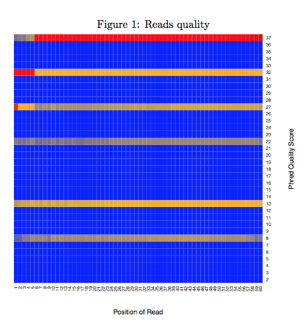
2.1 Reads quality
Reads quality is one of the basic reads level quality control methods. We plotted the distribution of a widely used Phred Quality Score at every position of sequence to measure the basic sequence quality of your data. Phred Quality Score was calculate by a python function ord(Q) − 33. Color in the heatmap represented frequency of this quality score observed at this position. Red represented higher frequency while blue was lower frequency. You may observe a decreasing of quality near the 3’end of sequence because of general degradation of quality over the duration of long runs. If the decreasing of quality influence the mappability(see “Bulk-cell level QC”) then the common remedy is to perform quality trimming where reads are truncated based on their average quality or you can trim serveal base pair near 3’end directly. If it doesn’t help, then you may consider re-sequence your samples.
2.2 Reads nucleotide composition
We assessed the nucleotide composition bias of a sample. The proportion of four different nucleotides was calculated at each position of reads. Theoretically four nucleotides had similar proportion at each position of reads. You may observe higher A/T count at 3’end of reads because of the 3’end polyA tail generated in sequencing cDNA libaray, otherwise the A/T count should be closer to C/G count. In any case, you should observe a stable pattern at least in the 3’end of reads. Spikes(un-stable pattern) which occur in the middle or tail of the reads indicate low sequence quality. You can trim serveral un-stable bases from the 3’end if low mappability(see “Bulk-cell level QC”) is also observed. If it doesn’t help, then you may consider your Drop-seq data poor quality. Note that the A/T vs G/C content can also greatly vary from species to species.

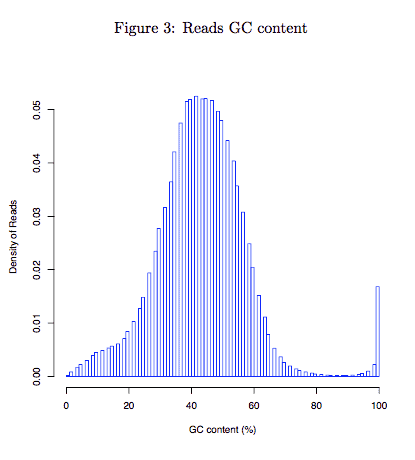
2.3 Reads GC content
Distribution of GC content of each read. This module measures the general quality of the library. If the distribution looks different from a single bell(too sharp or too broad) then there may be a problem with the library. Sharp peaks on an otherwise smooth distribution are normally the result of a specific contaminant (adapter dimers for example), which may well be picked up by the overrepresented sequences module. Broader peaks may represent contamination with a different species. If you get sharp peak or broder peak and also observe low mappability (see “Bulk-cell level QC”), you may consider reconstruct your library(redo the experiment).
3 Bulk-cell level QC
In the bulk-cell level QC step we measured the performance of total Drop-seq reads. In this step we did’t separate cell or remove “empty” cell barcodes, just like treated the sample as bulk RNA-seq sample.
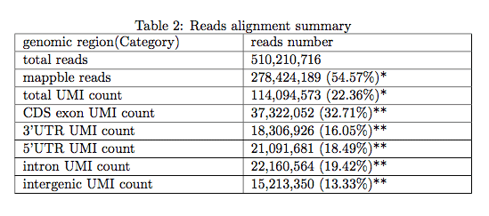
3.1 Reads alignment summary
The following table shows mappability and distribution of total Drop-seq reads. It measures the general quality of data as a RNA-seq sample. Low mappability indicates poor sequence quality(see “Reads level QC”) or library quality(caused by contaminant). High duplicate rate (low total UMI percentage observed, e.g. < 10%) indicate insufficient RNA material and Overamplification. In summary, if the percentage of "total UMI count" is less than 5%, users may consider reconstruct your library(redo the experiment), but first you should make sure you already trim the adapter and map your reads to the corresponded species(genome version). Note that UMI number was calculated by removing duplicate reads (which have identical genomic location, cell barcode and UMI sequences). Mappable reads was after Q30 filtering if Q30 filter function was turned on.
* the percentage was calculated by dividing total reads number
** the percentage was calculated by divding total UMI number
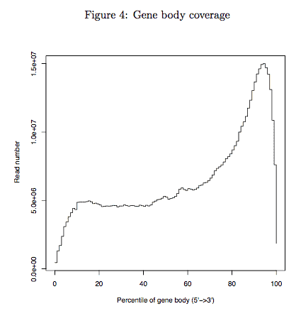
3.2 Gene body coverage
Aggregate plot of reads coverage on all genes. This module measures the general quality of Drop-seq data. Theoretically we observe a unimodal(single bell) distribution, but for Drop-seq sample an enrichment at 3’end is observed due to library preparation using oligo-dT primers. In any case you should observed a smooth distritbuion. If loss of reads or spike were observed in certain part of gene body (e.g. middle or 3’end of gene body), poor quality of your library was indicated. Especially when low mappability and high intron rate are also observed (see “Reads alignment summary” section).
4 Individual-cell level QC
In this step we focused on the quality of individual cell and distinguishing cell barcodes from STAMPs (single-cell transcriptomes attached to microparticles)
4.1 Reads duplicate rate distribution
Drop-seq technology has an innate advantage of detect duplicate reads and amplification bias because of the barcode and UMI information. This module displays the distribution of duplicate rate in each cell barcode and helps to discard cell barcodes with low duplicate rate (which usually caused by empty cell barcodes and ambient RNA). We plotted the distribution of duplicate rate in each cell barcode (though most of cell barcodes don’t contain cells, they still have RNA) and observed a bimodal distribution of duplicate rate. We set an option for you to discard cell barcodes with low duplicate rate in following steps. The vertical line represented the cutoff (duplicate rate >= 0.1) of discarding cell barcodes with low duplicate rate. You can adjust the cutoff and rerun Dr.seq if current cutoff didn’t separate two peaks from the distribution clearly (usually happened with insufficient sequencing depth). If the distribution didn’t show clear bimodal or you don’t want to discard cell barcodes according to duplicate rate, you can set cutoff to 0 to keep all cell barcodes.

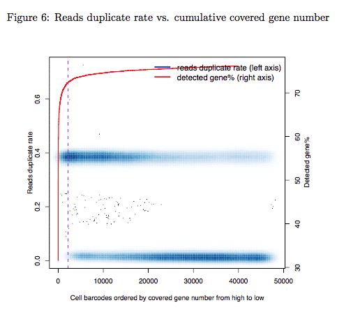
4.2 Reads duplicate rate vs. cumulative covered gene number
Reads duplicate rate versus cumulative covered gene numbers. This module measures whether each of your single cell was sequenced and was clearly separated from empty cell barcodes. Cell barcodes were ranked by the number of covered genes. The duplicate rate (y-axis, left side) was plotted as a function of ranked cell barcode. Red curve represented the number of genes covered by top N cell barcodes (y-axis, right side). N was showed by x-axis. Theoretically you will observed a “knee” on your cumulative curve (slope = 1 on the curve) and the cutoff of your selected STAMPs (dash line) should be close to the “knee”. The cutoff could be far away from the “knee” in some cases because you input too many cells and have insufficient sequencing depth, then you should adjust your cutoff (to the position you get enough STAMPs and sufficient reads count) and rerun Dr.seq. See the description of the paramter “select cell measure” in the Manual.
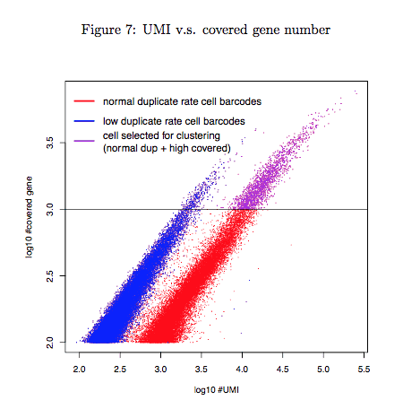
4.3 UMI vs. covered gene number
Covered gene number was plotted as a function of the number of UMI (i.e. unique read). This module measures the quality of Drop-seq experiment and helps to distinguish STAMPs from empty cell barcodes. We observed a clearly different pattern for two groups of cell barcodes with different reads duplicate rate (blue dots versus red and purple dots). Purple dots represented the selected STAMPs for the cell-clustering analysis. By default we select STAMPs with 1000 gene covered after discarding low duplicate cell barcodes. You might get few STAMPs according to this cutoff because of low sequencing depth and too many cells inputed. In this case you can adjust your cutoff or tell Dr.seq to directly select cell barcodes with highest reads count (see the description of the parameter “select cell measure”). Otherwise you may have to redo the experiment. Note that we use only STAMPs selected in this step for following analysis. The other cell barcodes are discarded.
4.4 Covered gene number distribution
Histogram of covered gene number of selected STAMPs. The module tell you whether the selected STAMPs have sufficient reads coverage. By default Dr.seq select STAMPs with cell barcodes with >= 1000 genes covered. If you select STAMPs with highest reads count (“select cell measure” = 2), then you should check this figure to make sure the STAMPs you select have enough gene covered. If most of your STAMPs have low covered gene number (e.g. < 100 gene covered), you can make your cutoff more stringent (e.g. select less cell barcodes with higher reads count) to make sure you get reliable STAMPs from empty cell barcodes.

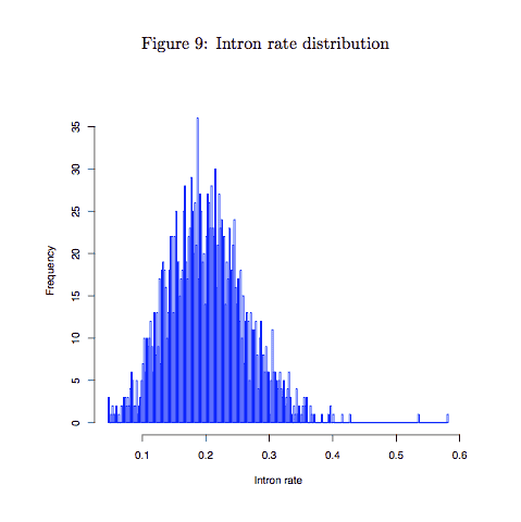
4.5 Intron rate distribution
Intron rate is a effective method to measure the quality of a RNA-seq sample. We plotted a histogram of intron rate of every STAMP barcodes to check whether reads from each STAMPs enriched in the exon region. High intron rate (e.g. >= 30%) indicates low quality of cDNA in each STAMPs (the low quality could be caused by different problem, for example contaminant). We suggest redo the Drop-seq experiment if most of selected STAMPs have high intron rate and low covered gene number (see “Covered gene number distribution” section). Intron rate was defined as intronUMInumber/(intron+exonUMInumber)
5 Cell-clustering level QC
This step composed by k-means clustering based on t-SNE dimentional reduction result and Gap statistics to determine best k.
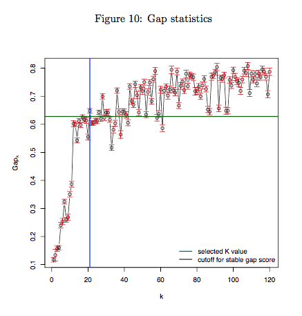
5.1 Gap statistics
We conducted a k-means clustering based on t-SNE dimensional reduction output to measure sample’s ability to be separated to different cell subtypes. Gap statistics was performed to determine the best k in k-means clustering. In general, decreasing pattern (usually k <= 2) is observed for pure cell type or cell line data, while increasing pattern with bigger k should be observed for mix cell types (or cell subtypes) data. If the cluster number predicted from the Gap statistics has great difference from what you expect, it indicated that your cells were not well characterized and separated by the Drop-seq experiment (because of the contaminant or the low capture efficiency of Droplets). We suggest considering poor quality of your Dropseq data and redo the experiments with refined protocol, because the general quality of Drop-seq data was not ensured when different cell types could even not be separated as expected.
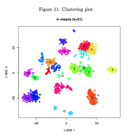
5.2 Cluster plot
Scatter plot represented visualization of t-SNE dimensional reduction output of selected STAMP barcodes. STAMP barcodes were colored according to the clustering result and cluster numbers were printed in the center of each cluster. This figure is mainly for visualization and help you to know how their data looked like. If you want to combine some small groups which are close to each other, you can use the cluster matrix (named “cluster.txt”) Dr.seq provided to conduct your own analysis.
5.2 Silhouette of clustering
Silhouette method is used to interprate and validate the consistency within clusters defined in previous steps. A poor Silhouette (e.g. average si < 0.2 ) score indicate that Drop-seq experiments(if not properly done) may not separate well the subpopulations of cells. If most of your clusters have poor Silhouette score, it may indicate a poor quality of your Drop-seq experiments.

Package download
Dr.seq is implemented by Python and freely avialable : Dr.seq.1.2.0.zip.
The lastest version is also in : https://bitbucket.org/Tarela/drseq.
Change log
v1.2.0 (2017.09.15) Bug fixed.
v1.1.3 (2016.08.17) Bug fixed.
v1.1.2 (2016.05.03) Add more detailed description in documents and manuals. set "remove_low_dup_cell" parameter to "0" (keep all cells) by default.
v1.1.1 (2016.03.25) Additional description in summary report was added according to bioinformatics revision.
v1.1.0 (2016.02.26) Silhouette score was added to Dr.seq as the last subsection of cell clustering step.
v1.0.2 (2016.01.18) The first released version, which generates the results of the paper.
Mapping software download
You can download mapping software from the official website(bowtie2,STAR).
Testing data download
testing barcode file: drseq_test_1.fastq.gz(size:294.3M) on YunBaidu or on Google Drive
testing reads file: drseq_test_2.fastq.gz (size:599.2M) on YunBaidu or on Google Drive
Q1: In the Manual section you use STAR as default parameter and generate example results with STAR, but you use bowtie2 for Quick start. What’s the difference?
A: We suggest using STAR as aligner mainly because of its speed. Drop-seq data requires huge amount reads to support thousand of single cell transcriptome to be detected, so the speed of alignment becomes a major factor we concern. In the quick start section we use bowtie2 because STAR requires > 30G memory for human genome, which is impossible for mac and small servers, while bowtie2 requires only 2~3G memory, which is suitable for almost all machines. Another reason is the mapping index for bowtie2 is much smaller than STAR (4G for bowtie2 index and 20G for STAR index), which is much easier to download.
Q2: I download your testing data but the result is not as clear as your example output. What’s the difference between testing data and the data you use for generating example?
A: We provide testing is only for users to get familiar with and see the flexibility of Dr.seq. The Drop-seq data we use to generate example contains 500 million total reads, and the total file size of 2 FASTQ files is greater than 200 gigabyte (200G), which is too big and not suitable for users to get started in a short time. To get users quickly familiar with Dr.seq, we provide a small dataset, which could be download and process very quickly. Note that the testing data is only for users to get familiar with Dr.seq in a very short time, so we don’t except this testing data to generate any meaningful results (For example, the duplicate rate distribution may not show different pattern because of low reads count, and there is not enough cells to provide a clear clustering pattern).
Q3: What should I do if I do want to generate your example output myself?
A: If you want to generate our example output yourself, you can download the corresponded Drop-seq data (accession ID mentioned in Quick Start section) and run Dr.seq with all default parameter (you can use both simple mode and standard mode with STAR as aligner, mm10 as genome version, see other default parameter from template configure file).
Q4: The published Drop-seq data I download is not FASTQ format, but .sra format. Also I only get a single .sra file. Where is my barcode and reads FASTQ file?
A: If you download the Drop-seq data we mentioned in Quick Start section from SRA, what you get is a single .sra file. You can transform and split the .sra file you download to barcode file and reads file in FASTQ format with free software called fastq-dump (from package SRA toolkit http://www.ncbi.nlm.nih.gov/Traces/sra/sra.cgi?view=software ). After you successfully installed SRA toolkit, Type command line:
$ fastq-dump.2.2.2 --split-files SRR1853178.sraThen the .sra file will be split to 2 FASTQ files, named as SRR1853178_1.fastq and SRR1853178_2.fastq. SRR1853178_1.fastq is barcode file and SRR1853178_2.fastq is reads file.
For other published Drop-seq data, you can read their description of data transform their published data to barcode.fastq and read.fastq for Dr.seq input. Note that sequences in barcode file should be composed with cell barcodes and UMIs. For each sequence, cell barcode part should locate before UMI part. For example, if the barcode in your fastq is AAAAAAAAAAAACCCCCCCC, then the cell_barcode of this reads is A*12 and the UMI is C*8. The length of cell barcode and UMI can be specified by two parameters, “cell_barcode_length” and “umi_length”.
Q5: I use Dr.seq to process my Drop-seq data with all default parameters, but the default parameter seems not suitable for my data. What should I do now?
A: To get initial sense of a new Drop-seq data, we suggest using Dr.seq with all default parameter (for example, simple mode). And after you get first feedback from Dr.seq output, you can specify the parameter and make Dr.seq suitable for your data. This time you can use aligned reads file in SAM format from the result of last run. To do this you need to input the location of aligned SAM file for “reads_file” in configure file (eg. “reads_file = /home/user/drseq1/mapping/defaultrun.sam”). The aligned SAM file is in the mapping/ folder in Dr.seq output and named as outname.sam. The original barcode file in FASTQ format should also be inputted. Use aligned reads file for Dr.seq can save you more than 80% of total time of last run.
Q6: There are too many parameters in standard mode, its too complicated for me to handle them.
A: Every parameter has its unique function and is required, but only some of them have great influence on the performande of Dr.seq. For example, you can change “select_cell_measure = 2” if you don’t like covered gene number to be the cutoff of STAMP barcodes. You can set “remove_low_dup_cell = 0” to include all cells if you don't believe low duplicate rate barcodes comes from bias. You can use DBSCAN for clustering if you don’t like our novel method for clustering.
If you don’t like change parameter in a configure file and do want to get feedback with “clicking a bottom”, we provide simple mode for you guys.
Q7: I know there are 2000 cells in my Drop-seq sample, but from the result of default Dr.seq, you only gave me 200 cells. How can I get my cells back?
A: By default we select STAMP barcodes with more than 1000 genes have reads covered. If your Drop-seq sample doesn’t have enough reads coverage, this cutoff may be too stringent for your sample. You can change the parameter “covergncluster” to get more or less STAMP barcodes. For those who want to get every cell back, we provide another STAMP selection method, that is, select STAMPs with topN highest reads count (UMI count). You can set “select_cell_measure = 2” and “topumicellnumber = 2000” if you put approximately 2000 real cells in your Drop-seq sample.
Q8: Why I get so many clusters from Dr.seq clustering result?
A: We designed a method to use kmeans + Gap statistics to cluster selected cells. To make there is enough cluster for kmeans to assign to small cell types, our method will generate slightly more cluster number than it suppose to be. We test the performande of our method on mouse retina cell Drop-seq data and simulated data, both gives satisfying result (see our paper). Users can combine nearby cluster from our provided clustering result, using optional kmeans+Gap statistics+maxSE to decide the number of cluster or using DBSCAN as clustering method if you don’t like the performande of our method.
Q9: I saw “error” in the analysis step, but Dr.seq still processed and “say” It’s DONE.

A: Here error is doesn’t means bug or crash down. It's mathematics error calculated by our dimensional reduction method: t-SNE.
There’s an easy way for you to check whether Dr.seq successfully generate the result. You can check summary/plots/ and summary/results/ folder for every results mentioned in our output list (see manual section for output list).
Q10: I don’t have pdflatex, and I don’t have root permission to install that. How can I get Dr.seq result?
A: Dr.seq will still process and generate all results if lack of pdflatex, you can check summary/plots/ folder and summary/results/ folder for everything you want. Also, if you do want the summary report, you can copy the whole summary/plots/ folder to another machine with pdflatex installed and type:
$ pdflatex outname_summary.texIn the plots/ folder to generate the summary report.
Q11: My sample doesn’t show clear bimodal about duplicate rate and I don’t believe low duplicate rate represent bias.
A: In the STAMP selection step in the original Drop-seq paper (Macosko, et al., 2015), they use topN cell barcodes with highest reads count, which contains almost NO cells with low duplicate rate. If you don’t like our method of removing low duplicate rate cells, you can turn off this function by set remove_low_dup_cell = 0”.
Q12: Dr.seq also provide PCA table and paired wise correlation table for all selected STAMP barcodes. What’s the usage of these two optional outputs?
A: We provide these two table incase some users don’t like our default workflow (PCA + t-SNE + kmeans + Gap stat) and do prefer PCA analysis only or distande correlation. So we provided these two optional outputs for those users to conduct further analysis based on their preferred intermediate results.