Quality control and analysis pipeline for parallel single cell transcriptome and epigenome data
Dr.seq2 is a QC and analysis pipeline for parallel single cell transcriptome and epigenome data. Dr.seq2 provides QC and analysis for three major data types: single cell transcriptome data (DrSeq part), Drop-ChIP data (DrChIP part) and scATAC-seq data (ATAC part). For single cell RNA-seq data, two additional step-by-step functions are included: 1. expression matrix generation for amounts of single cell RNA-seq datasets (GeMa step) and 2. cell clustering and analysis for the single cell expression matrix (comCluster step).
For different single cell datasets, Dr.seq2 uses sequencing files in FASTQ format or SAM format as input with relevant command. For transcriptome data, DrSeq uses two FASTQ files as standard input (one file contains the transcript reads and the other one contains cell barcode information, see our testing data and Manual section for more information) and provides four groups of QC measurements for given transcriptome data, including reads level, bulk-cell level, individual-cell level and cell-clustering level QC. Adapters are included in the pipeline for different parallel single cell RNA-seq technologies (MARS2Dr for MARS-seq data and 10x2Dr for 10x genomics data).
Here, we provide several examples to get you easily started on a Linux/MacOS system with only Python and R installed. To run Dr.seq2 with options specific to your data, see the Manual section for detailed directions.
Motivation:
An increasing number of single cell transcriptome and epigenome technologies, including Drop-ChIP and single cell ATAC-seq (scATAC-seq), have been recently developed as powerful tools to analyze the features of many individual cells simultaneously. However, the methods and software were designed for certain data types and only for single cell transcriptome data. A systematic approach for multiple types of data is needed to control data quality and to perform cell-to-cell heterogeneity analysis on these ultra-high-dimensional transcriptome and epigenome datasets.
Results:
We developed Dr.seq2, a Quality Control (QC) and analysis pipeline for multiple types of single cell transcriptome and epigenome data, including Drop-ChIP and scATAC-seq data. Application of this pipeline provides four groups of QC measurements and different analyses, including cell heterogeneity analysis. Dr.seq2 produced reliable results on published single cell transcriptome and epigenome datasets. Overall, Dr.seq2 is a systematic and comprehensive QC and analysis pipeline designed for parallel single cell transcriptome and epigenome data.
Workflow:
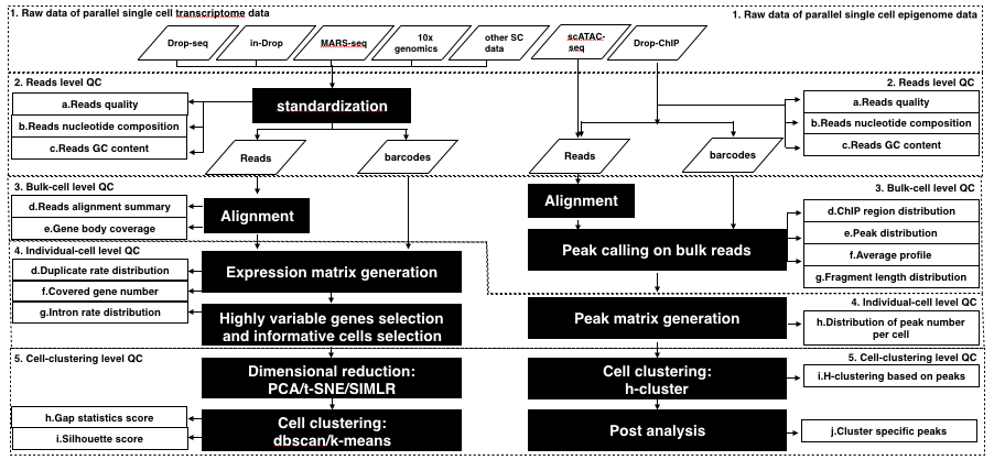
Flowchart illustrating the Dr.seq2 pipeline with default parameters. The workflow of the Dr.seq2 pipeline includes QC and analysis components for parallel single cell transcriptome and epigenome data. The QC component contains reads level, bulk-cell level, individual-cell level and cell-clustering level QC.
Citation:
This paper is under reversion.
Contact:
If you have any questions, suggestions, bug reports, etc, feel free to contact :Chengchen Zhao(1310780@tongji.edu.cn)
Installation
Prerequisite
1. python(version = 2.7)
2. R (version >= 2.14.1)
3. Dr.seq2 will generate a summary QC report if you have pdflatex installed, otherwise you only get a package of QC plots and analysis results in the summary.
Install Dr.seq2
Dr.seq2 uses Python's distutils tools for source installations. To install a source distribution of Dr.seq2, unpack the distribution zip file and open up a command terminal. Go to the directory where you unpacked Dr.seq2, and simply run the install script (We provide an example for installation in quick start section for users who feel confusing about the following description.):
$ python setup.py install
By default, the script will install python library and executable codes globally, which means you need to be root or administrator of the machine so as to complete the installation. Please contact the administrator of that machine if you want their help. If you need to provide a nonstandard install prefix, or any other nonstandard options, you can provide many command line options to the install script. Use the --help option to see a brief list of available options.
$ python setup.py install --prefix /home/DrSeq2
If you are not root user, you will be mentioned "permission denied" when you tried to install Dr.seq2 globally. Then you can use --prefix parameter to install Dr.seq2 to any directory you have write permission, you might need to add the install location to your PYTHONPATH and PATH environment variables. The process for doing this varies on each platform, but the general concept is the same across platforms.
Setup environment variable
PYTHONPATH
To set up your PYTHONPATH environment variable, you'll need to add the value PREFIX/lib/pythonX.Y/site-packages to your existing PYTHONPATH. In this value, X.Y stands for the major–minor version of Python you are using (in Dr.seq2 it should be 2.7; you can find this with sys.version[:3] from a Python command line). PREFIX is the install prefix where you installed Dr.seq2. If you did not specify a prefix on the command line, Dr.seq2 will be installed using Python's sys.prefix value.
For example, if you specify the parameter "--prefix /home/DrSeq2", you have to add /home/DrSeq2/lib/python2.7/site-packages to your PYTHONPATH (below is an example, DON’T add space near the equals sign).
$ export PYTHONPATH=/home/DrSeq2/lib/python2.7/site-packages:$PYTHONPATH
PATH
Just like your PYTHONPATH, you'll also need to add a new value to your PATH environment variable so that you can use the Dr.seq2 command line directly. Unlike the PYTHONPATH value, however, this time you'll need to add PREFIX/bin to your PATH environment variable. The process for updating this is the same as described above for the PYTHONPATH variable:
$ export PATH=/home/DrSeq2/bin:$PATH
To check your default PATH and PYTHONPATH, you can type:
$ echo $PATH
$ echo $PYTHONPATH
Automatically export PATH and PYTHONPATH
Feel bothering export environment variable every time ?
On Linux, using bash, you can include the new value in my PYTHONPATH by adding these lines
$ export PATH=/home/DrSeq2/bin:$PATHto your ~/.bashrc (or ~/.bash_profile). Then you export environment automatically and don’t need to export environment next time.
$ export PYTHONPATH=/home/DrSeq2/lib/python2.7/site-packages:$PYTHONPATH
Now you have Dr.seq2 installed on your computer, type "DrSeq --help" to check your installation.
Prepare gene annotation file
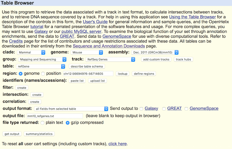
To use Dr.seq2 on transcriptome data, a gene annotation file with information regarding the location, name and composition of each gene is required. Dr.seq2 requires a gene annotation file with full information format (should be 16 coloumns) that can be downloaded from the UCSC genome browser http://genome.ucsc.edu/cgi-bin/hgTables. Below is an example for downloading the gene annotation file from the UCSC genome browser for the mm10 genome version.
We suggest using refseq genes for gene annotation, but you can also use annotations from other databases.
NOTE : The gene annotation files that used for transcriptome data and epigenome data are different. This gene annotation file (****_refgenes.txt) containing detail information in bed format for DrSeq to archive the bulk cell level QC part and generate gene expression. And the gene annotation file (****.refGene) used by DrChIP and ATAC is in a library format to archive the bulk cell level QC of epigenome data. Datails can be found in CEAS.
Prepare alignment software and build index
After Dr.seq2 is installed on the computer, single cell transcriptome data can be managed with a barcode file in FASTQ format and a reads file in SAM format (the reads file can be pre-aligned to the corresponding genome by any aligner). Using the full function of Dr.seq2, including the alignment step, users can input raw barcode files and raw reads files in FASTQ format to obtain QC and analysis results. The alignment software should be installed in the default PATH and the index should be built.
hisat2 (default), STAR and bowtie2 are accepted as aligners in Dr.seq2.
We have provided a download link for executable alignment software and a mapping index to save time and effort; see the following description and download section.
1. Install hisat2 and build hisat2 index
By default, we use hisat2 (version 2.1.1) as an aligner instead because hisat2 consumes as small memory as bowtie2; furthermore, it is as fast as STAR. Thus, we use hisat2 in the Quick Start section.You can download and compile hisat2 using the manual from the hisat2 website(https://ccb.jhu.edu/software/hisat2/index.shtml). hisat2 has its own index. After you finish installing hisat2, you can use the hisat2-build command to build the hisat2 index.
$ mkdir /home/user/hisat2_indexMore details can be found in the hisat2 website. After you finished building the index, you can use hisat2 as an aligner in Dr.seq2 simple mode.
$ cd /home/user/hisat2_index
$ hisat2-build mm10.fa mm10
1. Install STAR and build STAR index
We can also use STAR (version 2.5.0 or later) as alignment software given its speed and performance, but STAR also requires significant memory. To use STAR for alignment in Dr.seq2, first make sure that the memory of your server is greater than 40 G. Dr.seq2 will assess the total memory of your server before the alignment step if you use STAR as the alignment software (see the parameter description section for the corresponding parameter: checkmem). We do not recommend users to run STAR on a Mac computer.
To install STAR on you server, first you should download the STAR package and install STAR according to the instructions in the manual (github for STAR: https://github.com/alexdobin/STAR)
To help install STAR easily, we have provided a download link for executable STAR compiled in linux_x86_64 and macos_x86_64 system. See the download section of our webpage.
After you successfully install STAR or downloaded executable STAR, the next step is to build the STAR index.
To build a STAR index, first download the genome assembly file (typically a .fa file, you can easily download it from the UCSC genome browser http://genome.ucsc.edu/cgi-bin/hgTables Below is an example for downloading genome sequences in FASTA/fa format for the mm10 genome version.
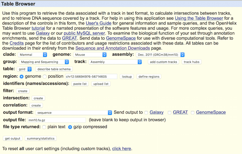
After the genome .fa file is downloaded, run a STAR build command to transform your .fa file into an index package (note that to you must create the directory before you build the STAR index).
$ mkdir /home/user/STAR_index# --runMode genomeGenerate: choose STAR build-index mode
$ STAR --runMode genomeGenerate --genomeDir /home/user/STAR_index --genomeFastaFiles /home/data/mm10.fa --runThreadN 8
# --genomeDir /home/user/STAR_index: name of directory where the STAR index is built
# --genomeFastaFiles /home/data/mm10.fa: the genome .fa file downloaded from UCSC
# --runThreadN 8: how many CPUs you want to use to generate the STAR index, this is a “speed up” parameter
The index is built, STAR can be used as an aligner in Dr.seq2 in the simple mode.
$ DrSeq simple -b SRR1853178_1.fastq -r SRR1853178_2.fastq -n GSM1626793_mouse_retina1 -g /home/user/annotation/mm10_refgenes.txt --maptool STAR --mapindex /home/user/STAR_index
Note that “STAR” is case sensitive in the --maptool parameter. Thus, Dr.seq2 will exit and let you input the correct alignment software if you want to perform the alignment step and input “--maptool star” as a parameter. The directory in which the STAR index is generated is the parameter of –mapindex.
Here, the parameter -g, --mapindex should be input with an absolute path (type pwd in command line to get the absolute path of your current directory).
2. Install bowtie2 and build bowtie2 index
If your server/computer does not have at least 40 G of memory (for example, you want to run Dr.seq2 on a Mac computer), you can use bowtie2 (version 2.2.6) as an aligner instead because bowtie2 consumes less memory (< 3 G memory for the human genome); however, it is slower.
You can download and compile bowtie2 using the manual from the bowtie2 website(http://bowtie-bio.sourceforge.net/bowtie2/manual.shtml).
If you do not want to or have trouble installing bowtie2 and building the bowtie2 index, we have provided a download link for executable bowtie2 compiled in linux_x86_64 and macos_x86_64 system and the bowtie2 index for different species and genome versions. See the download section of our webpage.
Bowtie2 has its own index. After you finish installing bowtie2, you can use the bowtie2-build command to build the bowtie2 index.
$ mkdir /home/user/bowtie2_index
$ cd /home/user/bowtie2_index
$ bowtie2-build mm10.fa mm10
After you finish building the index, you can use bowtie2 as an aligner in Dr.seq2 simple mode.
$ DrSeq simple -b SRR1853178_1.fastq -r SRR1853178_2.fastq -n GSM1626793_mouse_retina1 -g /home/user/annotation/mm10_refgenes.txt --maptool bowtie2 --mapindex /home/user/bowtie2_index/mm10# --mapindex /home/user/bowtie2_index/mm10: absolute path of bowtie2 index. Note that the genome version of the index should corresponded to the annotation file. If you have an index file looks like: /home/user/bowtie2_index/mm10.1.bt2, the red part is the one you should input here.
4. Prepare peak calling software
Macs14 is used for peak calling in Dr.seq2 on Drop-ChIP data and single cell ATAC data. You can download MACS14 from here.$ cd MACS-1.4.2-1More details about MACS see MACS web page
$ python setup.py install --prefix /home/
$ export PYTHONPATH=/home/lib/python2.6/site-packages:$PYTHONPATH
$ export PATH=/home/bin:$PATH
Install pdflatex
For mac user, you can get download "MacTex" from http://www.tug.org/mactex/. After downloading the package MacTex.pkg from http://tug.org/cgi-bin/mactex-download/MacTeX.pkg, you just double click to install MacTex and get the pdflatex.
For linux user, you can type
$ apt-get install texlive-allto install pdflatex on your server/computer.
Note that the installation of pdflatex on both mac and linux requires root privilege.
Install SIMLR
SIMLR(Single-cell Interpretation via Multi-kernel LeaRning) is a novel similarity-learning framework, which learns an appropriate distance metric from the data for dimension reduction, clustering and visualization. Dr.seq2 integrated SIMLR as an dimension reduction method.
To run it successfully, these two steps should be finished before the Dr.seq2 installation
1) Required R libraries. SIMLR requires 2 R packages to run, namely the Matrix package (see https://cran.r-project.org/web/packages/Matrix/index.html) to handle sparse matrices and the parallel package (see https://stat.ethz.ch/R-manual/R-devel/library/parallel/doc/parallel.pdf) for a parallel implementation of the kernel estimation.
2) External C code. We make use of an external C program during the computations of SIMLR. The code is located in the R directory in the file projsplx_R.c. In order to compite the program, one needs to run on the shell the command:
$ cd Dr.seq2.1.2/lib/RscriptThen install DrSeq following the manual.
$ R CMD SHLIB -c projsplx_R.c
 $ cd ../../
 $ sudo python setup.py install
Note: if there are issues when compiling the .c file, try to remove the pre-compiled files (i.e., projsplx_R.o and projsplx_R.so).
Usage of Dr.seq2
Dr.seq2 provides QC and analysis for three major data types: single cell transcriptome data (DrSeq part), Drop-ChIP data (DrChIP part) and scATAC-seq data (ATAC part). For single cell RNA-seq data, two additional step-by-step functions are included: 1. expression matrix generation for amounts of single cell RNA-seq datasets (GeMa step) and 2. cell clustering and analysis for the single cell expression matrix (comCluster step). For different parallel single cell RNA-seq technologies, input data are standardized for DrSeq part.
Run Dr.seq2 on single cell transcriptome data
Standard mode and simple mode
The command in Dr.seq2 for running transcriptome data is DrSeq. DrSeq provides two modes. You can edit and design a parameter complex suitable for your data with the standard mode, but a configure file must be generated and edited before using DrSeq. Simple mode is designed for a convenient and quick start. With this mode, DrSeq can be run with a simple command line, but only major parameters can be edited with this mode.
Simple mode
The simple mode is described in the quick start section. In simple mode, only the input data, output name, mapping tool, annotation and mapping index must be specified with a command line, and DrSeq will generate QC and analysis reports with all default parameters.
All parameters used in the simple mode are also used in the standard mode and will be described below:
$ DrSeq simple [-h] -b BARCODE -r READS -n NAME[--cellbarcoderange CBR] [--umirange UMIR] [-g GA][--maptool {STAR,bowtie2}] [--checkmem {0,1}][--mapindex MAPINDEX] [--thread P] [-f] [--clean][--select_cell_measure {1,2}][--remove_low_dup_cell {0,1}]
Type$ DrSeq simple -hfor detailed description of all major parameters of simple mode.
Standard mode
In standard mode, you can edit all parameters and customize DrSeq for your data.
First, you should generate a configure file according to the template configure file (we will describe how to find and edit template configure files below) by typing:
$ DrSeq gen your_config_name.conf
Now you have generated a configure file (named your_config_name.conf in the example) according to the template configure file. If you open the configure file generated, you will find all changeable parameters listed with the pattern "parameter = value" (for example, barcode_file = SRR1853178_1.fastq) and the corresponding description in the bottom of each panel (starts with "#").
We use a Python package called "ConfigParser" to parse the configure file, which requires a specific pattern of the input configure file. Thus, users must take certain precautions when editing the configure file:
1. Do not edit the description lines (the lines starting with "#"); keep these lines that start with "#"
2. Keep the pattern "parameter = value" for parameter lines. Do not remove the value for any parameter line if you do not have a specific value for it. Keep the space next to the equal sign.
Now, you can edit your configure file and customize it for your Drop-ChIP data (If you do not have suitable initial parameters , you can run DrSeq in simple mode with only major parameters changed and edit other parameters according to the DrSeq output. Then, you can re-run DrSeq with updated parameters. Re-running DrSeq takes only 20% of the total time, see the FAQ section).
After you finish editing the configure the file, you can use standard mode to run DrSeq with your edited configure file input.
DrSeq run -c your_edit_config.conf -f --clean# -c your_edited_config.conf: name of your input configure file. The configure file should be generated using DrSeq gen mode or copied from another DrSeq run. The major parameters (parameters with "[required]" in the description line), including input file location, gene annotation file location, alignment software and mapping index, corresponding to the software should be specified by the user.
# -f: force_overwrite: DrSeq will overwrite the output results if the output folder already exists when -f is added, otherwise DrSeq will exit.
# --clean: DrSeq will remove intermediate result if --clean is added.
DIY template configure file to save your specific parameters
If it is too complicated to edit the configure file for the same parameters for each DrSeq run, the template configure file can be edited in the DrSeq package before DrSeq is installed to save changes to major parameters (for example, edit gene annotation file, alignment software, mapping index and other parameters) in the template configure file. If you have already installed DrSeq, the template configure file can be edited and installed again.
First, you should find the template configure file. It is located in the "lib/Config/" folder of the DrSeq package and named "DrSeq_template.conf" (do NOT change the file name of the template configure file).
After you find the template configure file, you can edit it to change the commonly used parameters. For example, if you change the parameter "gene_annotation = /data/mm10_refgenes.txt" and then re-install DrSeq, the configure file you generate next time will always have "gene_annotation = /data/mm10_refgenes.txt". Thus, you do not need to edit it again. Generally, we suggest editing gene_annotation, mapping_software_main and mapindex. You can also change cell_barcode_range if your barcode looks different from the published Drop-ChIP data (12 bp for cell barcode, 8 bp for UMI). Editing the template configure file is similar to editing the generated configure file.
Both standard mode and simple mode will use the edited the template configure file.
Full parameter description
Below is the description of all changeable parameters. The value after equal sign is the default (suggested) value of the parameter. [required] means this parameter should be specified for different samples.
A more convenient way is to read the same version in configure file while you are editing configure file and specify parameters.
General
# In General panel we describe major parameters of DrSeq
barcode_file = /home/user/SRR1853178_1.fastq
# [required]barcode_file : Fastq file only, by default, every barcode in fastq file consist of 20 bp including 12bp cell barcode(1-12bp) and 8bp UMI(13-20bp). Cell barcode should locate before UMI, the range of cell barcode and UMI can be defined below.
# eg: /home/user/SRR1853178_1.fastq
cell_barcode_range = 1:12
umi_range = 13:20
# cell_barcode_range/umi_range: range of cell barcode and UMI, (see the annotation of barcoe_fastq). By default they are 1:12,13:20, respectively
reads_file = /home/user/SRR1853178_2.fastq
# [required]reads_file: Accept raw sequencing file (fastq) or aligned file(sam), file type is specified by extension. (regard as raw file and add mapping step if .fastq, regard as aligned file and skip alignment step if .sam), sam file should be with header.
# eg: /home/user/SRR1853178_2.fastq
outputdirectory = /home/user/GSM1626793_mouse_retina1/
# [required]outputdirectory: (absolute path) Directory for all result. Default is current dir "." if user left it blank , but not recommended.
# eg: /home/user/GSM1626793_mouse_retina1/
outname = GSM1626793_mouse_retina1
# [required]outname: Name of all your output results, your results will looks like outname.pdf, outname.txt
# eg: GSM1626793_mouse_retina1
gene_annotation = /home/user/annotation/mm10_refgenes.txt
# [required]gene_annotation: (absolute path) Gene model in full text format, download from UCSC genome browser,
# eg: /yourfolder/mm10_refgenes.txt (absolute path, refseq version recommended )
png_for_dot = 0
# png_for_dot: Only works for dotplots in individual cell QC. Set 1 to plot dotplots in individual cell QC in png format, otherwise they will be plotted in pdf format. The format of other plots is fixed to pdf.
# Make sure your Rscript is able to generate PNG plots if you turn on this function.
Step1_Mapping
# In Mapping panel we describe parameters related to the alignment of reads file
mapping_software_main = hisat2
# [required if reads file is FASTQ format]mapping_software_main: name of your mapping software, choose from hisat2, STAR and bowtie2 (case sensitive), hisat2 (STAR or bowtie2) should be installed in your default PATH
checkmem = 1
# checkmem: (only take effect when mapping_software_main = STAR) DrSeq will check your total memory to make sure its greater 40G if you choose STAR as mapping tool. We don't suggest running STAR on Mac. You can turn off (set 0) this function if you prefer STAR regardless of your memory (which may cause crash down of your computer)
mapping_p = 8
# mapping_p: Number of alignment threads to launch
mapindex = /home/user/hisat2_index
# [required if reads file is FASTQ format]mapindex: Mapping index of your alignment tool, absolute path,
# Mapping index should be built before you run this pipeline, note that STAR and bowtie2 use different index type (see STAR/bowtie2 document for more details.).
# For STAR, mapindex should be the absolute path of the folder you built STAR index, this parameter will be directly used as the mapping index parameter of STAR
# eg: /mnt/Storage3/mapping_idnex/mm10.star
# For bowtie2, mapindex should be absolute path of index filename prefix (minus trailing .X.bt2).this parameter will be directly used as the mapping index parameter of bowtie2
# eg: /mnt/Storage3/mapping_index/mm10.bowtie2/mm10 (then under your folder /mnt/Storage3/mapping_index/mm10.bowtie2/ there should be mm10.1.bt2, mm10.rev.1.bt2 .... ),
q30filter = 1
# q30filter: Use q30 criteria (Phred quality scores) to filter reads in samfile, set this parameter to 1(default) to turn on this option, set 0 to turn off
Step2_ExpMat
# In ExpMat panel we describe parameters related to generating expression matrix
filterttsdistande = 0
# filterttsdistande: Whether discard reads far away from transcript terminal site (TTS), set 1 to turn on this function, default is 0 (not use).
ttsdistande = 400
# ttsdistande: Default filter distande is 400bp (discard reads 400bp away from TTS), only take effect when filterttsdistande = 1 is set
covergncutoff = 100
# covergncutoff: Only plot cell barcodes with more than 100 (default) genes covered in the dotplots in individual-cell QC step.
# Note that this parameter is only for visualization of QC report and convenience of following analysis, because too many cell_barcodes will influence users' interpretation of the QC report.
# Users can change this parameter when the drop-seq sample doesn’t have enough coverage/read depth
# To determine "STAMP barcodes" from cell barcodes for clustering, users can change parameter in [Step4_Analysis] "covergncluster"
duplicate_measure = 2
# duplicate_measure: method to consider duplicate reads in each cell barcodes when generate expression matrix,
# 1: combine duplicate reads with same UMI and same genomic location (position and strand)
# 2(default): only consider UMI (combine duplicate reads with same UMI)
# 3: only consider genomic location only (combine duplicate reads with same genomic location)
# 0: do not remove (combine) duplicate reads (keep all duplicate reads, skip combination step)
umidis1 = 0
# umidis1: only take effect when duplicate_measure = 1 or 2, ignore this parameter if duplicate_measure = 0 or 3
# Set 1: if two reads from same cell barcode have same genomic location (chrom,position,strand) and their UMI distande <= 1, regard them as duplicate reads and combine them
# Set 0 (default): regard them as duplicate reads only when their UMI distande = 0 and have genomic location
# By default this function is turned off
Step3_QC
# In QC panel we describe parameters related to quality control and STAMP barcodes selection
select_cell_measure = 1
# select_cell_measure: Method to select real cells from cell_barcodes, choose from 1 or 2
# 1 (default): Cell_barcodes with more than 1000 genes covered are selected as real cells for following analysis including dimentional reduction and clustering, cutoff of covered gene number (1000, default) is determined in parameter "covergncluster"
# 2: Top 1000 cell_harcodes with highest UMI count will be selected as real cells, number of highest UMI cell (1000, default) is determined in parameter "topumicellnumber". Suitable for Drop-ChIP sample with known cell number
covergncluster = 1000
# covergncluster: cell_barcodes with more than 1000 (default) genes covered will be selected as STAMP barcodes for clustering
# This parameter takes effect only when "select_cell_measure" is set to 1
topumicellnumber = 1000
# topumicellnumber: Top 1000(default) cell_barcodes with highest UMI count will be selected as STAMP barcodes for clustering
# This parameter takes effect only when "select_cell_measure" is set to 2
remove_low_dup_cell = 0
# remove_low_dup_cell: A group of cell barcodes have almost no duplicate reads, which show clearly different pattern from STAMP barcodes, we set an option to remove these cell_barcodes
for analysis step.
# # Choose from 0 or 1, set 1 to turn on this function (remove low duplicate rate cell_barcodes), set 0 (default) to turn off (keep low duplicate rate cell_barcodes)
# Removing low duplicate cells maybe not so effective when sequencing depth is not enough.
non_dup_cutoff = 0.1
# non_dup_cutoff: Only take effect when remove_low_dup_cell is turned on. Cutoff of low-duplicate cell_barcode (default is 0.1), a cell_barcode will be defined as low-duplicate cell_barcode if its duplicate rate < 0.1. Duplicate rate for each cell_barcode is defined as (#total_reads - #UMI)/#total_reads
Step4_Analysis
# In analysis panel we describe parameters related to dimensional reduction, highly variable gene selection and clustering
dimensionreduction_method = 1
# dimensionreduction_method : Method for dimension reduction
# chosse from 1(default),2,3
# 1(default) : t-SNE
# 2 : SIMLR
# 3 : PCA
highvarz = 1.64
# highvarz: Cutoff for high variande selection. In the first step we divide all genes to 20 groups based on average expression level across all individual cells. Then in each group we select genes whose z-normalized CV (var/mean) >= 1.64 (default, corresponding to pvalue =0.05)
selectpccumvar = 0.5
# selectpccumvar: Select topN PC until they explain 50% (default is 0.5, eg. 0.3 for 30% variande) of total variande. Then conduct 2 dimensional t-SNE based on selected PCs
pctable = 1
# pctable: choose from 0(default) and 1, you can turn on this function(set 1) to output a 2 column table for PC1 v.s PC2
# This paramter is designed for users who prefer and conduct following analysis based on PCA output
# 0(default): Do not output PCA result, only output PCA + 2 dimensional t-SNE result (see document for more details)
# 1: Output PC1 v.s. PC2 table in addition to t-SNE result.
cortable = 1
# cortable: Choose from 0(default) and 1, you can turn on this function(set 1) to output a cell to cell correlation matrix
# Correlation is based on log scale TPM (transcript per million reads).
# User can turn on this function to generate cell to cell correlation matrix for custom analysis
clustering_method = 1
# clustering_method: Method for cluster cells based on t-SNE output
# Choose from 1(default), 2, 3 and 4.
# 1(default): k-means, use Gap statistics followed by our "first stable Gap" method to determine k
# 2: k-means, but use Gap statistics followed by traditional "Tibs2001SEmax" method to determine k (Tibshirani et al (2001))
# 3: k-means with custom determined k, k value is defined in following parameter "custom_k", this option is designed for users who know the number of subgroup of the drop-seq sample
# 4: (make sure your R enviroment has library "fpc" installed) Use dbscan as clustering method, the (eps) parameter is defined in following parameter "custom_d"
maxknum = 100
# maxknum: Maximum k number for gap statistics, only take effect when clustering_method = 1 or 2
custom_k = 5
# custom_k: Only take effect when clustering_method = 3, cells will be clustered to N group based on t-SNE result according to user determined k
custom_d = 2
# custom_d: Only take effect when clustering_method = 4, refer to the parameter "eps"(Reachability distande, see Ester et al. (1996)) of dbscan. By default we set it to 2 according to the orginal Drop-ChIP paper, but it varies a lot between different datasets.
rdnumber = 1007
# rdnumber: Set initial random number to keep your result reproducible
Run Dr.seq2 on Drop-ChIP data
Standard mode and simple mode
The command in Dr.seq2 for running transcriptome data is DrChIP
Now, you can run DrChIP to generate QC and analysis reports of your Drop-ChIP data with two-part sequencing data input containing barcode information and reads information. DrChIP provides two modes. You can edit and design a parameter complex suitable for your data with the standard mode, but a configure file must be generated and edited before using DrChIP. Simple mode is designed for a convenient and quick start. With this mode, DrChIP can be run with a simple command line, but only major parameters can be edited with this mode.
Simple mode
The simple mode is described in the quick start section. In simple mode, only the input data, output name, mapping tool, annotation and mapping index must be specified with a command line, and DrChIP will generate QC and analysis reports with all default parameters.
All parameters used in the simple mode are also used in the standard mode and will be described below:
$ DrChIP simple [-h] -1 FASTQ_1 -2 FASTQ_2 -b BARCODE_FILE --barcode_file_range_1 BARCODE_FILE_RANGE_1 --barcode_file_range_2 BARCODE_FILE_RANGE_2 --barcode_range_1 BARCODE_RANGE_1 --barcode_range_2 BARCODE_RANGE_2 -n NAME -g GA -s SPECIES -l CL [--maptool MAPTOOL] [--mapindex MAPINDEX] [-p P] [-X X] [--trim5 TRIM5] [-f] [--clean] [--cell_cutoff CELL_CUTOFF] [--peak_cutoff PEAK_CUTOFF]Type
$ DrChIP simple -hfor detailed description of all major parameters of simple mode.
Standard mode
In standard mode, you can edit all parameters and customize DrChIP for your data.
First, you should generate a configure file according to the template configure file (we will describe how to find and edit template configure files below) by typing:
$ DrChIP gen your_config_name.conf
Now you have generated a configure file (named your_config_name.conf in the example) according to the template configure file. If you open the configure file generated, you will find all changeable parameters listed with the pattern "parameter = value" (for example, barcode_file = SRR1853178_1.fastq) and the corresponding description in the bottom of each panel (starts with "#").
We use a Python package called "ConfigParser" to parse the configure file, which requires a specific pattern of the input configure file. Thus, users must take certain precautions when editing the configure file:
1. Do not edit the description lines (the lines starting with "#"); keep these lines that start with "#"
2. Keep the pattern "parameter = value" for parameter lines. Do not remove the value for any parameter line if you do not have a specific value for it. Keep the space next to the equal sign.
Now, you can edit your configure file and customize it for your Drop-ChIP data (If you do not have suitable initial parameters , you can run DrChIP in simple mode with only major parameters changed and edit other parameters according to the DrChIP output. Then, you can re-run DrChIP with updated parameters.
After you finish editing the configure the file, you can use standard mode to run DrChIP with your edited configure file input.
DrChIP run -c your_edit_config.conf -f --clean# -c your_edited_config.conf: name of your input configure file. The configure file should be generated using DrChIP gen mode or copied from another DrChIP run. The major parameters (parameters with "[required]" in the description line), including input file location, gene annotation file location, alignment software and mapping index, corresponding to the software should be specified by the user.
# -f: force_overwrite: DrChIP will overwrite the output results if the output folder already exists when -f is added, otherwise DrChIP will exit.
# --clean: DrChIP will remove intermediate result if --clean is added.
DIY template configure file to save your specific parameters
If it is too complicated to edit the configure file for the same parameters for each DrChIP run, the template configure file can be edited in the DrChIP package before DrChIP is installed to save changes to major parameters (for example, edit gene annotation file, alignment software, mapping index and other parameters) in the template configure file. If you have already installed DrChIP, the template configure file can be edited and installed again.
First, you should find the template configure file. It is located in the "lib/Config/" folder of the DrChIP package and named "DrChIP_template.conf" (do NOT change the file name of the template configure file).
After you find the template configure file, you can edit it to change the commonly used parameters. For example, if you change the parameter "gene_annotation = /data/mm10_refgenes.txt" and then re-install DrChIP, the configure file you generate next time will always have "gene_annotation = /data/mm10_refgenes.txt". Thus, you do not need to edit it again. Generally, we suggest editing gene_annotation, mapping_software_main and mapindex. Editing the template configure file is similar to editing the generated configure file.
Both standard mode and simple mode will use the edited the template configure file.
Full parameter description
Below is the description of all changeable parameters. The value after equal sign is the default (suggested) value of the parameter. [required] means this parameter should be specified for different samples.
A more convenient way is to read the same version in configure file while you are editing configure file and specify parameters.
General
# In General panel we describe major parameters of DrChIP
fastq_1 =
fastq_2 =
barcode_range_1 = 1:8
barcode_range_2 = 12:19
barcode_file =
barcode_file_range_1 = 5:12
barcode_file_range_2 = 49:56
outputdirectory =
outname =
gene_annotation = /home/user/annotation/mm9.refGene
chrom_length = /home/user/annotation/mm9.len
species =
# [required]fastq_1 : Fastq file only, by default, every barcode in fastq file.
# [required]fastq_2: Accept raw sequencing file (fastq) or aligned file(sam), file type is specified by extension. (regard as raw fileand add mapping step if .fastq, regard as aligned file and skip alignment step if .sam), sam file should be with header
# [required]barcode_range_1: The location range of cell barcode in the read1. For example, if the barcode in your fastq isAAAAAAAAXXXXXXXXXXXXX, then the cell_barcode of this reads is A 1:8
# [required]barcode_range_2: The location range of cell barcode in the read2.
# [required]barcode_file: The file containing the sequence of barcode pool.
# [required]barcode_file_range_1: The location range of cell barcode in the given barcode read1.
# [required]barcode_file_range_2: The location range of cell barcode in the given barcode read2.
# [required]outputdirectory: (absolute path) Directory for all result. default is current dir "." if user left it blank , but notrecommended.
# [required]outname: Name of all your output results, your results will looks like outname.pdf, outname.txt
# [required]gene_annotation: (absolute path) gene annotation file downloaded from CEAS eg: /yourfolder/mm9_refgenes.txt (absolutepath, refseq version recommended ). "/Users/Drseq/Desktop/mm9_refgenes.txt" is absolute path, while "~/Desktop/mm9_refgenes.txt" is NOT
# [required]chrom_length : The annotation file containing the length of each chromsome.
# [required]species : The species of the input data. By now, only 'mm' and 'hs' are acceptable. 'mm' : mouse.'hs': human.
Step1_Mapping
# In Mapping panel we describe parameters related to the alignment of reads file
mapping_software = bowtie2
p = 8
mapindex = /home/user/bowtie2_index
q30filter = 1
X = 1000
trim5 = 23
# [required]mapping_software: name of your mapping software, choose from STAR and bowtie2 (case sensitive), bowtie2(STAR) should be
installed in your default PATH, see Manual
# p: Number of alignment threads to launch alignment software
# [required]mapindex: Mapping index of your alignment tool, absolute path.
# Mapping index should be built before you run this pipeline, note that STAR and bowtie2 use different index type(see STAR/bowtie2
document for more details.).
# For bowtie2, mapindex should be absolute path of index filename prefix (minus trailing .X.bt2).this parameter will be directly
used as the mapping index parameter of bowtie2
# eg: /mnt/Storage3/mapping_index/mm9.bowtie2/mm9 (then under your folder /mnt/Storage3/mapping_index/mm9.bowtie2/ there should
be mm9.1.bt2, mm9.rev.1.bt2 .... ),
# q30filter: Use q30 criteria (Phred quality scores) to filter reads in samfile, set this parameter to 1(default) to turn on this
option, set 0 to turn off. Default is 1
# X : maximum fragment length (bowtie2 parameter)
# trim5 : trim
Step2_QC
# In QC panel we describe parameters related to peak calling
peak_calling_cutoff = 1e-5
# peak_calling_cutoff: threshold for macs2 peak calling
Step3_CellClustering
# In Step3_CellClustering panel we describe parameters related to cell clustering and post analysis
peak_extend_size = 5000
max_barcode_num = 1152
cut_height = 1
cell_cutoff = 20
peak_cutoff = 20
# peak_extend_size: size of peak extension to measure the peak existence in each cell.
# max_barcode_num : the max number of your input barcode, refering to your barcode input.(default is the 1152 -- calculated from the barcode we provide.)
# cut_height : height for cutting tree.
# cell_cutoff : discard the peaks containing cells less than
# peak_cutoff : discard the cells containing peaks less than
Run Dr.seq2 on single cell ATAC-seq data
Simple mode for scATAC-seq data
You can also run Dr.seq2 pipeline to generate QC and analysis reports of your single cell ATAC-seq(scATAC) datasets.
Here, we provide an example of our simple mode on combined published scATAC-seq datasets (GSM1596255~GSM1596350,GSM1596735~GSM1596830 and GSM1597119~GSM1597214).
$ ATAC -i DrSeq2_scATAC -o scATAC -g hs --layout pair --geneannotation /PATHtoRefGene/hg19.refGene --cell_cutoff 5 --peak_cutoff 5 -C 3
Full parameter description
# Full parameter description for ATAC.
-i INPUT_FILES, --input_files=INPUT_FILES input mapped reads file of single cell ATAC-seq. Sam/Bam files are supported,multiple files should seperate by comma.This parameter is required.
-o OUTNAME, --outname=OUTNAME output name.This parameter is required.Default is 'out'.
-g GENOME_TYPE, --genome_type=GENOME_TYPE genome_type for effective genome size. It can be shortcuts:'hs' for human (2.7e9), 'mm' for mouse (1.87e9) Default:hs
-p PVALUE, --pvalue=PVALUE p-value cutoff for peak detection. DEFAULT: 1e-5.
-c CUT_HEIGHT, --cut_height=CUT_HEIGHT height for cutting tree. DEFAULT: 0. Ignored when -C set.
-C CLUSTER_NUMBER, --cluster_number=CLUSTER_NUMBER Given cluster numbers. DEFAULT: 2.
--qfilter=QFILTER whether filter out reads that are bad according to sequencing quality
--layout=LAYOUT pair-end sequencing or single-end sequencing.'pair' strands for pair-end sequencing.'single' strands for single-end sequencing.
--geneannotation=GENEANNOTATION gene annotation file for CEAS.
--chrom_length=CHROM_LENGTH chrom length file for bw file generation.
--cell_cutoff=CELL_CUTOFF discard the peaks containing cells less than
--peak_cutoff=PEAK_CUTOFF discard the cells containing peaks less than
Output of Dr.seq2
We provide a QC and analysis report pdf file for each kind of data as examples.
| data type | filename |
|---|---|
| single cell transcriptome data(10x genomics) | jurkat_293t_50_50_summary.pdf on YunBaidu or on Google Drive |
| Drop-ChIP data | H3K4me2_140226_07_summary.pdf on YunBaidu or on Google Drive |
| single cell ATAC-seq data | scATAC_H1_GM12878_K562_summary.pdf on YunBaidu or on Google Drive |
OUTPUT LIST
| file name | description |
|---|---|
| scATAC_peaks.bed on YunBaidu or on Google Drive | Combined peaks for scATAC-seq datasets |
| scATACpeakMatrix.txt on YunBaidu or on Google Drive | Covered region matrix for each single cell |
| scATAC_cluster1_cells.txt on YunBaidu or on Google Drive | Cells in each cluster |
| scATAC_cluster1_specificpeak.bed on YunBaidu or on Google Drive | Cell type specific peaks for each cluster |
| scATAC_cluster_with_silhouette_score.txt on YunBaidu or on Google Drive | cell clustering results with Silhouette Score |
| scATAC_H1_GM12878_K562_summary.pdf on YunBaidu or on Google Drive | Dr.seq2 QC report for scATAC-seq datasets |
The details of QC measurements is shown blow:
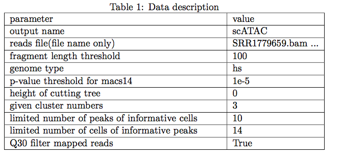
1 Data description
Table 1 mainly describe the input file and mapping and analysis parameters.
2 Bulk-cell level QC
In the bulk-cell level QC step we measured the performance of total scATAC-seq reads. In this step we did’t separate cell or remove "empty" cell barcodes, just like treated the sample as bulk ATAC-seq sample.
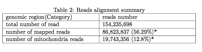
2.1 Reads alignment summary
The following table shows mappability total scATAC-seq reads. It measures the general quality of data as a high thoughput sequencing data. Low mappability indicates poor sequence quality or library quality(caused by contaminant). In summary, if the percentage of "number of mapped reads" is less than 5%, users may consider reconstruct your library(redo the experiment), but first you should make sure you already trim the adapter and map your reads to the corresponded species(genome version).
* the percentage was calculated by dividing total number of reads
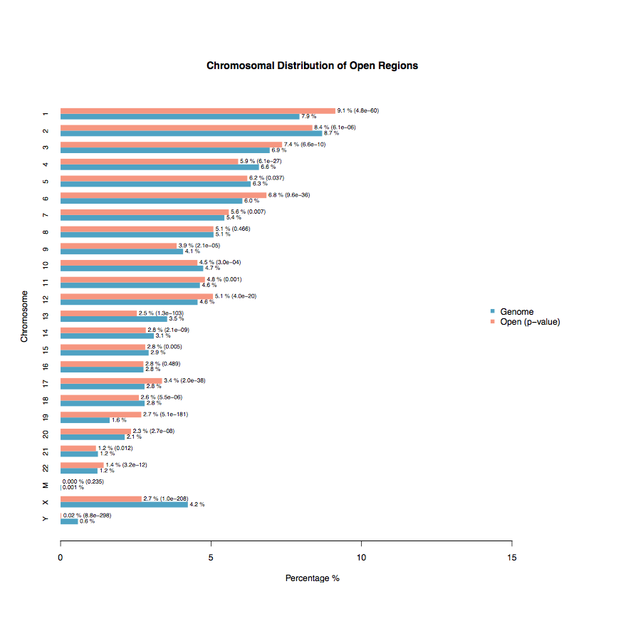
2.2 Chromosomal Distribution of ChIP Regions
The blue bars represent the percentages of the whole tiled or mappable regions in the chromosomes (genome background) and the red bars shows the percentages of the whole ChIP. These percentages are also marked right next to the bars. P-values for the significance of the relative enrichment of ChIP regions with respect to the gnome background are shown in parentheses next to the percentages of the red bars.
2.3 Peaks over Chromosomes
Barplot show ChIP regions distributed over the genome along with their scores or peak heights. The line graph on the top left corner illustrates the distribution of peak heights (or scores). The red bars in the main plot ChIP regions in the input BED file. The x-axis of the main plot represents the actual chromosome sizes.

2.4 Average profile on different genomic regions
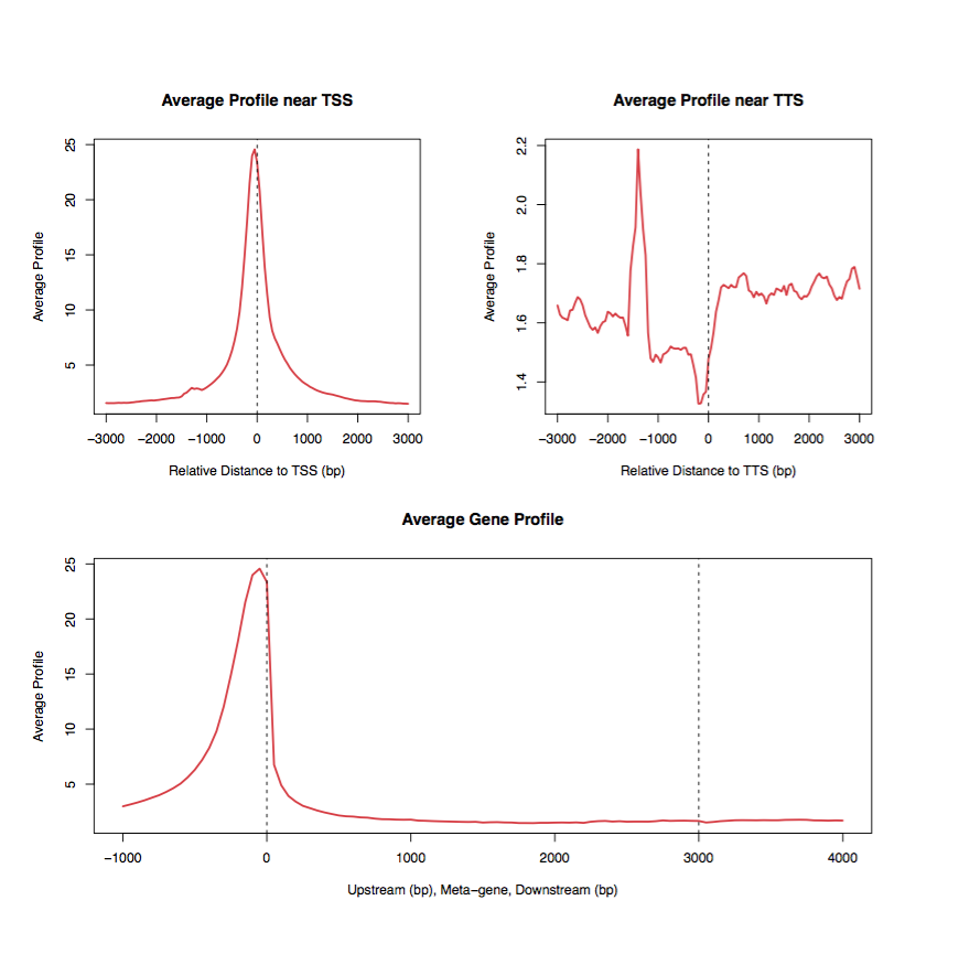
Average profiling within/near important genomic features. The panels on the first row display the average ChIP enrichment signals around TSS and TTS of genes, respectively. The bottom panel represents the average ChIP signals on the meta-gene of 3 kb.
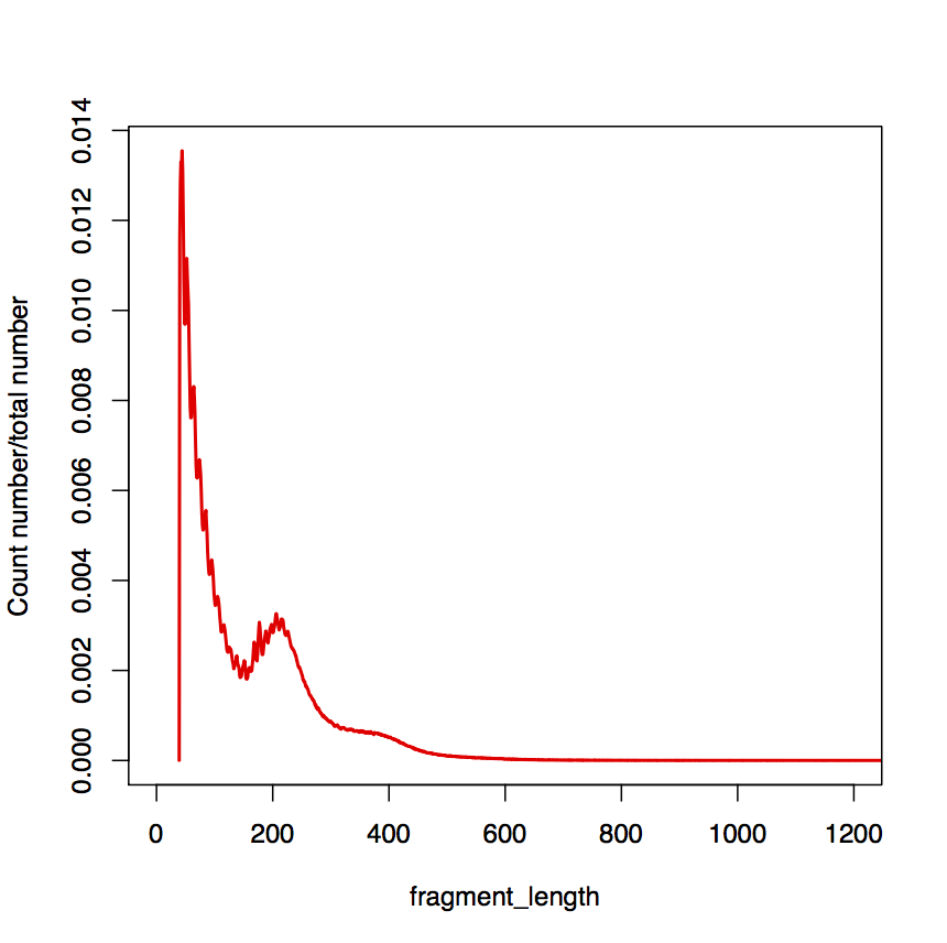
2.5 Distribution of fragment length numbers (excluded fragments in mitochondria)
ATAC-seq indicated factor occupancy and nucleosome positions with periodicity fragment length distribution.
3 Individual-cell level QC
In this step we focused on the quality of individual cell and distinguishing cell barcodes from STAMPs (single-cell transcriptomes attached to microparticles)
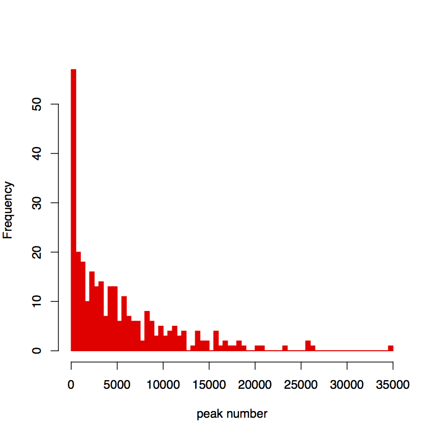
3.1 Distribution of peak numbers per cell
To measure whether the cell is informative for post-analysis, peak number per each cell is calculated, The cells with small number of peaks indicated the limited informative of cells.
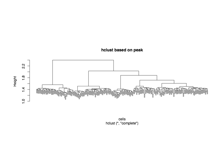
4 Cell-clustering level QC
This step composed by h-clustering based on macs14 peaks.
4.1 Cell clustering
We conducted a h-cluster based on macs14 peaks to measure sample’s ability to be separated to different cell subtypes.
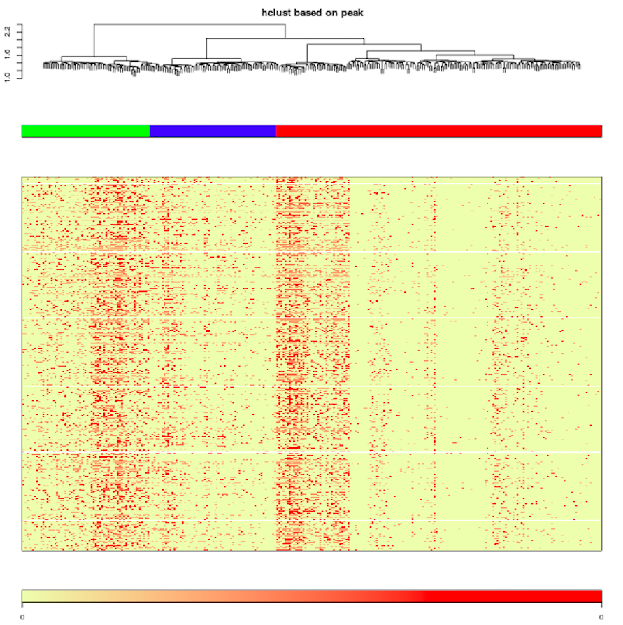
4.2 Clustering heatmap
Cell Clustering tree and peak region in each cell. The upper panel represents the hieratical clustering results based on each single cell. The second panel with different colors represents decision of cell clustering. The bottom two panels (heatmap and color bar) represent the ”combined peaks” occupancy of each single cell.
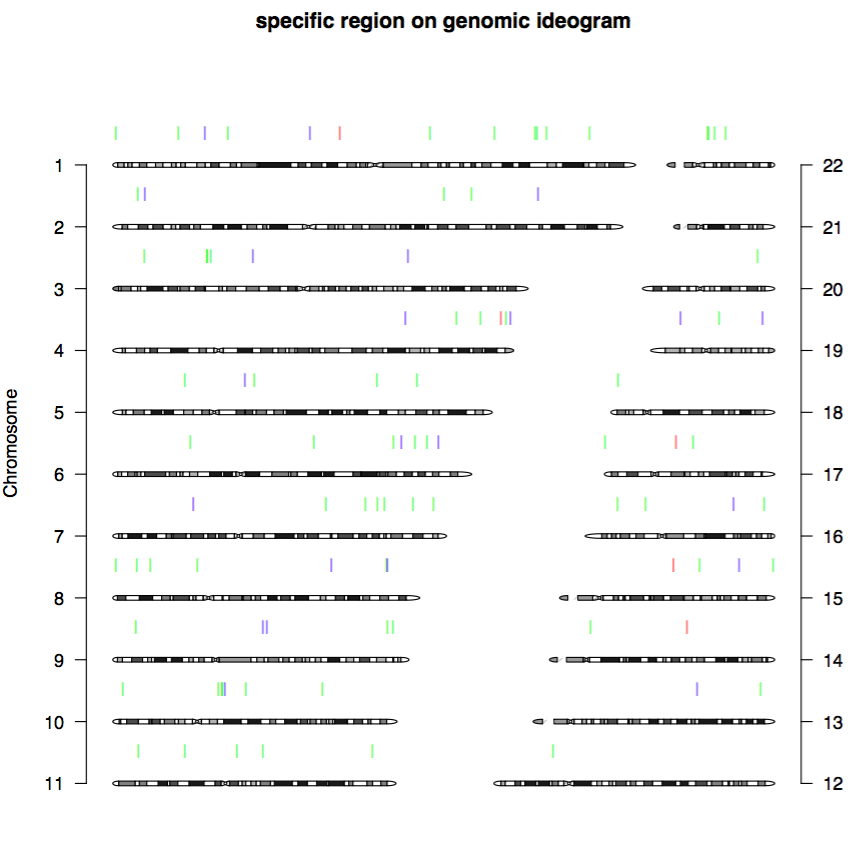
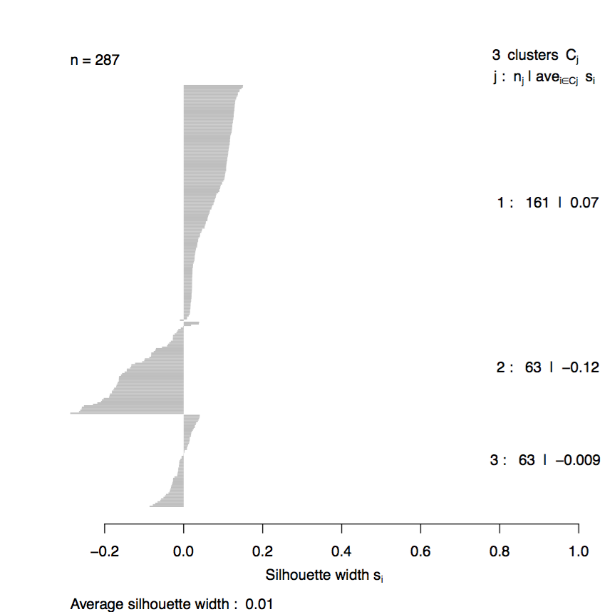
4.3 Ideogram of cluster specific regions Silhouette of clustering
Cluster specific regions in each chromosome. Specific peaks for different cell clusters are marked by different colors and ordered according to genomic loci.
4.4 Silhouette of clustering
Silhouette method is used to interprate and validate the consistency within clusters defined in previous steps. A poor Silhouette (e.g. average si < 0.2 ) score indicate that scATAC-seq experiments(if not properly done) may not separate well the subpopulations of cells. If most of your clusters have poor Silhouette score, it may indicate a poor quality of your scATAC-seq experiments.
Package download
Dr.seq2 is implemented by Python and freely avialable : Dr.seq2.1.2.
Our previous version (Dr.seq) is still available in http://www.tongji.edu.cn/~zhanglab/drseq/.
The lastest version is also in : https://github.com/ChengchenZhao/DrSeq2.
Change log
v2.1.2 (2017.09.15) [Dr.seq2] New Function:add hisat2 as a new mapping software option. Bug fixed:duplicate_measure=2.
v2.1.1 (2017.08.02) [Dr.seq2] Bug fixed:Reads-level QC legend.
v2.1.0 (2017.05.04) [Dr.seq2] Change "ChIP region" to "Open region" for scATAC reports.
v2.0.2 (2017.02.16) [Dr.seq2] Bug fixed for PCA in few single cell RNA-seq datasets analysis.
v2.0.1 (2017.02.15) [Dr.seq2] Bug fixed.
v2.0.0 (2017.01.25) [Dr.seq2] new version released.
v1.1.3 (2016.08.17) [Dr.seq] Bug fixed.
v1.1.2 (2016.05.03) [Dr.seq] Add more detailed description in documents and manuals. set "remove_low_dup_cell" parameter to "0" (keep all cells) by default.
v1.1.1 (2016.03.25) [Dr.seq] Additional description in summary report was added according to bioinformatics revision.
v1.1.0 (2016.02.26) [Dr.seq] Silhouette score was added to Dr.seq2 as the last subsection of cell clustering step.
v1.0.2 (2016.01.18) [Dr.seq] The first released version, which generates the results of the paper.
Testing data download
testing scATAC file: DrSeq2_scATAC_test.tar.gz on YunBaidu or on Google Drive(size:509.6M)
Q1: I download your testing data but the result is not as clear as your example output. What’s the difference between testing data and the data you use for generating example?
A: We provide testing is only for users to get familiar with and see the flexibility of Dr.seq2. The scATAC data we use to generate Dr.seq2 report contains ~500 million total reads, and the total file size is greater than 10G gigabyte (10G), which is too big and not suitable for users to get started in a short time. To get users quickly familiar with Dr.seq2, we provide a small dataset, which could be download and process very quickly. Note that the testing data is only for users to get familiar with Dr.seq2 in a very short time, so we don’t expect this testing data to generate any meaningful results.
Q2: The published Drop-ChIP data I download is not FASTQ format, but .sra format. Also I only get a single .sra file. Where is my barcode and reads FASTQ file?
A: If you download the Drop-seq data we mentioned in Quick Start section from SRA, what you get is a single .sra file. You can transform and split the .sra file you download to barcode file and reads file in FASTQ format with free software called fastq-dump (from package SRA toolkit http://www.ncbi.nlm.nih.gov/Traces/sra/sra.cgi?view=software ). After you successfully installed SRA toolkit, Type command line:
$ fastq-dump.2.2.2 --split-files SRR1853178.sraThen the .sra file will be split to 2 FASTQ files, named as SRR1853178_1.fastq and SRR1853178_2.fastq. SRR1853178_1.fastq is barcode file and SRR1853178_2.fastq is reads file.
For other published single cell transcriptome data, you can read their description of data standardized their published data to barcode.fastq and read.fastq for Dr.seq2 input. Note that sequences in barcode file should be composed with cell barcodes and UMIs. For each sequence, cell barcode part should locate before UMI part. For example, if the barcode in your fastq is AAAAAAAAAAAACCCCCCCC, then the cell_barcode of this reads is A*12 and the UMI is C*8. The range of cell barcode and UMI can be specified by two parameters, "cell_barcode_range" and "umi_range".
Q3: I have successfuly installed Dr.seq2 on my mac, but why there are still errors when I using Dr.seq2 on transcriptome data?
A: You may use the dimensional reduction method "SIMLR" before install it in Dr.seq2. At first, ensure you installed all the required tools and R packages. For mac that using Mavericks and lower version of system, "gfortran", which is needed for the installation of some R package, is missing at the moment. Try these commends to install the "gfortran" before you install some R packages.
curl -O http://r.research.att.com/libs/gfortran-4.8.2-darwin13.tar.bz2
sudo tar fvxz gfortran-4.8.2-darwin13.tar.bz2 -C /
Q4: I use Dr.seq2 to process my Drop-ChIP data with all default parameters, but the default parameter seems not suitable for my data. What should I do now?
A: To get initial sense of a new Drop-ChIP data, we suggest using Dr.seq2 with all default parameter (for example, simple mode). And after you get first feedback from Dr.seq2 output, you can specify the parameter and make Dr.seq2 suitable for your data. This time you can use aligned reads file in SAM format from the result of last run. To do this you need to input the location of aligned SAM file for "reads_file" in configure file (eg. "reads_file = /home/user/DrSeq2/mapping/defaultrun.sam"). The aligned SAM file is in the mapping/ folder in Dr.seq2 output and named as outname.sam. The original barcode file in FASTQ format should also be inputted. Use aligned reads file for Dr.seq2 can save you more than 80% of total time of last run.
Q5: There are too many parameters in standard mode, its too complicated for me to handle them.
A: Every parameter has its unique function and is required, but only some of them have great influence on the performande of Dr.seq2. For example, when apply Dr.seq2 on single cell transcriptome data, you can change "select_cell_measure = 2" if you don’t like covered gene number to be the cutoff of STAMP barcodes. You can set "remove_low_dup_cell = 0" to include all cells if you don't believe low duplicate rate barcodes comes from bias. You can use DBSCAN for clustering if you don’t like our novel method for clustering.
If you don’t like change parameter in a configure file and do want to get feedback with "clicking a bottom", we provide simple mode for you guys.
Q6: Why I get so many clusters from Dr.seq2 clustering result for single cell transcriptome data?
A: We designed a method to use kmeans + Gap statistics to cluster selected cells. To make there is enough cluster for kmeans to assign to small cell types, our method will generate slightly more cluster number than it suppose to be. We test the performande of our method on mouse retina cell Drop-ChIP data and simulated data, both gives satisfying result (see our paper). Users can combine nearby cluster from our provided clustering result, using optional kmeans+Gap statistics+maxSE to decide the number of cluster or using DBSCAN as clustering method if you don’t like the performande of our method.
Q7: I saw "error" in the analysis step for single cell transcriptome data, but Dr.seq2 still processed and "say" It’s DONE.
A: Here error is doesn’t means bug or crash down. It's mathematics error calculated by our dimensional reduction method: t-SNE.
There’s an easy way for you to check whether Dr.seq2 successfully generate the result. You can check summary/plots/ and summary/results/ folder for every results mentioned in our output list (see manual section for output list).
Q8: I don’t have pdflatex, and I don’t have root permission to install that. How can I get Dr.seq2 result?
A: Dr.seq2 will still process and generate all results if lack of pdflatex, you can check summary/plots/ folder and summary/results/ folder for everything you want. Also, if you do want the summary report, you can copy the whole summary/plots/ folder to another machine with pdflatex installed and type:
$ pdflatex outname_summary.texIn the plots/ folder to generate the summary report.